The ancient oriental game of Go has long been considered a grand challenge for artificial intelligence. For decades, computer Go has defied the classical methods in game tree search that worked so successfully for chess and checkers. However, recent play in computer Go has been transformed by a new paradigm for tree search based on Monte-Carlo methods. Programs based on Monte-Carlo tree search now play at human-master levels and are beginning to challenge top professional players. In this paper, we describe the leading algorithms for Monte-Carlo tree search and explain how they have advanced the state of the art in computer Go.
1. Introduction
Sequential decision making has been studied in a number of fields, ranging from optimal control through operations research to artificial intelligence (AI). The challenge of sequential decision making is to select actions that maximize some long-term objective (e.g., winning a game), when the consequences of those actions may not be revealed for many steps. In this paper, we focus on a new approach to sequential decision making that was developed recently in the context of two-player games.
Classic two-player games are excellent test beds for AI. They provide closed micro-worlds with simple rules that have been selected and refined over hundreds or thousands of years to challenge human players. They also provide clear benchmarks of performance both between different programs and against human intelligence.
In two-player games such as chess, checkers, othello, and backgammon, human levels of performance have been exceeded by programs that combine brute force tree-search with human knowledge or reinforcement learning.22
For over three decades however, these approaches and others have failed to achieve equivalent success in the game of Go. The size of the search space in Go is so large that it defies brute force search. Furthermore, it is hard to characterize the strength of a position or move. For these reasons, Go remains a grand challenge of artificial intelligence; the field awaits a triumph analogous to the 1997 chess match in which Deep Blue defeated the world champion Garry Kasparov.22
The last five years have witnessed considerable progress in computer Go. With the development of new Monte-Carlo algorithms for tree search,12,18 computer Go programs have achieved some remarkable successes,12,15 including several victories against top professional players. The ingredients of these programs are deceptively simple. They are provided with minimal prior knowledge about the game of Go, and instead they acquire their expertise online by simulating random games in self-play. The algorithms are called Monte-Carlo tree search (MCTS) methods, because they build and expand a search tree while evaluating the strength of individual moves by their success during randomized play.
2. The Game of Go
The game of Go is an ancient two-player board game that originated in China. It is estimated that there are 27 million Go players worldwide. The game of Go is noted for its simple rules but many-layered complexity.
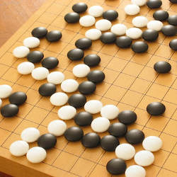
The black and white players alternate turns. On each turn, they place a single stone of their corresponding color on an N × N board. The standard board size is 19 × 19, but smaller boards, namely, boards of size 9 × 9 and 13 × 13 are also played to a lesser extent in competitive play, for study, and also for computer Go development. A group is a connected set of stones (using 4-connectivity) of the same color. A liberty is an empty location that is adjacent to a group. A group is captured when it has no more liberties. The stones of a captured group are removed from the board. It is illegal to play suicidal moves that would result in self-capture. A group is termed dead when it is inevitable that it will be captured. The aim of the game is to secure more territory than the other player. Informally, territory describes the empty locations on the board that are unambiguously controlled by one player. The game ends when both players pass, at which time the two players count their scores. Each player receives one point for every location of territory that they control, and one point for each captured stone. White receives a bonus, known as komi, compensating for the fact that black played first. The player with the highest score wins. The precise scoring details vary according to regional rules; however, all major scoring systems almost always lead to the same result. Figure 1 shows a complete game of 9 × 9 Go.
The handicap is the number of compensation stones that the black player is allowed to place on the board before alternating play. The goal of handicap is to allow players of different strength to play competitively. “Even games” are games with handicap 0 and a komi of 7.5 (the komi can vary according to regional rules).
The ranks of amateur Go players are ordered by decreasing kyu and then increasing dan, where the difference in rank corresponds to the number of handicap stones required to maintain parity. Professional players are ordered by increasing dan, on a second scale (Figure 2). The title “top professional” is given to a professional player who has recently won at least one major tournament.
 2.2. Go: A grand challenge for AI
Since the introduction of Monte-Carlo tree search in 2006, the ranks of computer Go programs have jumped from weak kyu level to the professional dan level in 9 × 9 Go, and to strong amateur dan level in 19 × 19 Go (see Section 5).
The game of Go is difficult for computer programs for a number of reasons. First, the combinatorial complexity of the game is enormous. There are many possible moves in each turn: approximately 200 in Go, compared to 37 for chess. Furthermore, the length of a typical game is around 300 turns, compared to 57 in chess. In fact, there are more than 10170 possible positions in Go, compared to 1047 in chess, and approximately 10360 legal move sequences in Go, compared to 10123 in chess.22
Another factor that makes Go challenging is the long-term influence of moves: the placement of a stone at the beginning of the game can significantly affect the outcome of the game hundreds of moves later. Simple heuristics for evaluating a position, such as counting the total material advantage, have proven to be very successful in chess and checkers. However, they are not as helpful in Go since the territorial advantage of one player is often compensated by the opponent’s better strategic position. As a result, the best known heuristic functions evaluate positions at the beginner level. All these make the game of Go an excellent challenge for AI techniques, since a successful Go program must simultaneously cope with the vast complexity of the game, the long-term effects of moves, and the importance of the strategic values of positions. Many real-world, sequential decision-making problems are difficult for exactly the same reasons. Therefore, progress in Go can lead to advances that are significant beyond computer Go and may ultimately contribute to advancing the field of AI as a whole. One support for this claim is the fact that Monte-Carlo tree search, which was originally introduced in Go, has already started to achieve notable successes in other areas within AI.20,25
3. Monte-Carlo Tree Search
The common approach used by all the strongest current computer Go programs is Monte-Carlo tree search (MCTS).12 In this section, we first introduce game trees and discuss traditional approaches to game tree search. Next, we discuss how Monte-Carlo techniques can be used to evaluate positions. Finally, we introduce the UCT (upper confidence bounds on trees) strategy,18 which guides the development of the search tree toward positions with large estimated value or high uncertainty.
We begin by discussing search algorithms for two-player games in general. In such games, there are two players, whom we shall call Black and White. The players move in an alternating manner, and the games are assumed to be deterministic and to be perfect information. Determinism rules out games of chance involving, for example, dice throws or shuffled cards in a deck. Perfect information rules out games where the players have private information such as cards that are hidden from the other players. More specifically, perfect information means that, knowing the rules of the game, each player can compute the distribution of game outcomes (which is a single game outcome, if deterministic) given any fixed future sequence of actions. Another way of putting this latter condition is to say that both players have perfect knowledge of the game’s state. In board games such as Go, chess, and checkers, disregarding subtleties such as castling restrictions in chess and ko rules in Go, the state is identical to the board position, that is, the configuration of all pieces on the board.
The rules of the game determine the terminal states in which the game ends. There is a reward associated with each terminal state, which determines as to how much Black earns if the game ends in that state. There are no intermediate rewards, that is, the reward associated with each nonterminal state is zero. The goal of Black is to get the highest final reward, while the goal of White is to minimize Black’s reward.
A game tree organizes the possible future action sequences into a tree structure. The root of the tree represents the initial state (and the empty action sequence), while each other node represents some nonempty, finite action sequence of the two players. Each finite action sequence leads deter-ministically to a state, which we associate with the node corresponding to that action sequence (Figure 3).
Note that the same state can be associated with many nodes of the tree, because the same state can often be reached by many distinct action sequences, known as transpositions. In this case, the game can be represented more compactly by a directed acyclic graph over the set of states.
The optimal value of a game tree node is the best possible value that the player at that node can guarantee for himself, assuming that the opponent plays the best possible counter-strategy. The mapping from the nodes (or states) to these values is called the optimal value function. Similarly, the optimal action value of a move at a node is defined to be the optimal value of the child node for that move.
If the optimal values of all children are known, then it is trivial to select the optimal move at the parent: the Black (White) player simply chooses the move with the highest (lowest) action-value. Assuming that the tree is finite, the optimal value of each node can be computed by working backward from the leaves, using a recursive procedure known as minimax search.
While minimax search leads to optimal actions, it is utterly intractable for most interesting games; the computation is proportional to the size of the game tree, which grows exponentially with its depth. A more practical alternative is to consider a subtree of the game tree with limited depth. In this case, computation begins at the leaves of the subtree. The (unknown) true optimal values at the leaf nodes are replaced with values returned by a heuristic evaluation function. If the evaluation function is of sufficiently “high quality,” the action computed is expected to be near-optimal. The computation can be sped up by various techniques, the most well-known being α − β pruning, which is often used together with iterative deepening.
The evaluation function is typically provided by human experts, or it can be tuned either using supervised learning based on a database of games or using reinforcement learning and self-play.22 Programs based on variants of minimax search with α − β pruning have outperformed human world champions in chess, checkers, and othello.22
In some games of interest, for example in the game of Go, it has proven hard to encode or learn an evaluation function of sufficient quality to achieve good performance in a minimax search. Instead of constructing an evaluation function, an alternative idea is to first construct a policy (sometimes called a playout policy) and then to use that policy to estimate the values of states. A policy is a mapping from states to actions; in other words, a policy determines the way to play the game. Given a policy pair (one policy for each player, which if symmetric can be represented by a single policy), a value estimate for a state s can be obtained by simulation: start in state s and follow the respective policies in an alternating manner from s until the end of the game, and use the reward in the terminal state as the value of state s. In some games, it is easier to estimate the value indirectly by simulation, that is, it may be easier to come up with a simple policy that leads to good value estimates via simulation than to estimate those values directly.
A major problem with the approach described so far is that it can be very sensitive to the choice of policy. For example, a good policy may choose an optimal action in 90% of states but a suboptimal action in the remaining 10% of states. Because the policy is fixed, the value estimates will suffer from systematic errors, as simulation will always produce a single, fixed sequence of actions from a given state. These errors may often have disastrous consequences, leading to poor evaluations and an exploitable strategy.
Monte-Carlo methods address this problem by adding explicit randomization to the policy and using the expected reward of that policy as the value estimate. The potential benefit of randomization is twofold: it can reduce the influence of systematic errors and it also allows one to make a distinction between states where it is “easy to win” (i.e., from where most reasonable policy pairs lead to a high reward terminal state) and states where it is “hard to win.” This distinction pays off because real-world opponents are also imperfect, and therefore it is worthwhile to bias the game toward states with many available winning strategies. Note that the concepts of “easy” and “hard” do not make sense against a perfect opponent.
When the policy is randomized, computing the exact expected value of a state under the policy can be as hard as (or even harder than) computing its optimal value. Luckily, Monte-Carlo methods can give a good approximation to the expected value of a state. The idea is simply to run a number of simulations by sampling the actions according to the randomized policy. The rewards from these simulations are then averaged to give the Monte-Carlo value estimate of the initial state.
In detail, the value of action a in position s0 (the root of the game tree) is estimated as follows. Run N simulations from state s0 until the end of the game, using a fixed randomized policy for both players. Let N(a) be the number of these simulations in which a is the first action taken in state s0. Let W(a) be the total reward collected by Black in these games. Then, the value of action a is estimated by
 .
.
The use of Monte-Carlo methods in games dates back to 1973 when Widrow et al.24 applied Monte-Carlo simulation to blackjack. The use of Monte-Carlo methods in imperfect information and stochastic games is quite natural. However, the idea of artificially injecting noise into perfect information, deterministic games is less natural; this idea was first considered by Abramson.2 Applications of Monte-Carlo methods to the game of Go are discussed by Bouzy and Helmstetter.6
Monte-Carlo tree search (MCTS) combines Monte-Carlo simulation with game tree search. It proceeds by selectively growing a game tree. As in minimax search, each node in the tree corresponds to a single state of the game. However, unlike minimax search, the values of nodes (including both leaf nodes and interior nodes) are now estimated by Monte-Carlo simulation (Figure 4).
In the previous discussion of Monte-Carlo simulation, we assumed that a single, fixed policy was used during simulation. One of the key ideas of MCTS is to gradually adapt and improve this simulation policy. As more simulations are run, the game tree grows larger and the Monte-Carlo values at the nodes become more accurate, providing a great deal of useful information that can be used to bias the policy toward selecting actions which lead to child nodes with high values. On average, this bias improves the policy, resulting in simulations that are closer to optimal. The stronger the bias, the more selective the game tree will be, resulting in a strongly asymmetric tree that expands the highest value nodes most deeply. Nevertheless, the game tree will only typically contain a small subtree of the overall game. At some point, the simulation will reach a state that is not represented in the tree. At this point, the algorithm reverts to a single, fixed policy, which is followed by both players until a terminal state is reached, just like Monte-Carlo simulation. This part of the simulation is known as a roll-out.
More specifically, MCTS can be described by four phases. Until a stopping criterion is met (usually a limit on available computation time), MCTS repeats four phases: descent, roll-out, update, and growth. During the descent phase, initiated at the current state s0, MCTS iteratively selects the highest scoring child node (action) of the current state. The score may simply be the value of the child node, or may incorporate an exploration bonus (see next section). At the end of the descent phase, that is, upon reaching a leaf node of the current tree, the roll-out phase begins, where just like in Monte-Carlo simulation, a fixed, stochastic policy is used to select legal moves for both players until the game terminates. At the end of the roll-out, the final position is scored to determine the reward of Black. In the update phase, the statistics (number of visits and number of wins) attached to each node visited during descent are updated according to the result of the game. In the growth phase, the first state visited in the roll-out is added to the tree, and its statistics are initialized.
3.4. Upper confidence bounds on trees (UCT)
An extremely desirable property of any game-tree-search algorithm is consistency, that is, given enough time, the search algorithm will find the optimal values for all nodes of the tree, and can therefore select the optimal action at the root state. The UCT algorithm is a consistent version of Monte-Carlo tree search.
If all leaf value estimates were truly the optimal values, one could achieve consistency at the parent nodes by applying greedy action selection, which simply chooses the action with the highest value in each node. If all descendants of a given node have optimal value estimates, then greedy action selection produces optimal play from that node onward, and therefore simulation will produce an optimal value estimate for that node. By induction, the value estimate for all nodes will eventually become optimal, and ultimately this procedure will select an optimal action at the root.
However, the value estimates are not usually optimal for two reasons: (i) the policy is stochastic, so there is some inherent randomness in the values, and (ii) the policy is imperfect. Thus, going with the action that has the highest value estimate can lead to suboptimal play, for example, if the value of the optimal action was initially underestimated. Therefore, occasionally at least, one must choose actions that look suboptimal according to the current value estimates.
The problem of when and how to select optimal or suboptimal actions has been extensively studied in the simplest of all stochastic action selection problems. These problems are known as multi-armed bandit problems.a Each game ends after the very first action, with the player receiving a stochastic reward that depends only on the selected action. The challenge is to maximize the player’s total expected reward, that is, quickly find the action with the highest expected reward, without losing too much reward along the way. One simple, yet effective strategy is to always select the action whose value estimate is the largest, with an optimistic adjustment that takes account of the uncertainty of the value estimate. This way, each action results either in an optimal action or in a reduction of the uncertainty associated with the value estimate of the chosen action. Thus, suboptimal actions cannot be chosen indefinitely.
The principle of always choosing the action with the highest optimistic value estimate is known as the “principle of optimism in the face of uncertainty” and was first proposed and studied by Lai and Robbins.19 A simple implementation of this idea, due to Auer et al.,3 is to compute an upper confidence bound (UCB) for each value estimate, using Hoeffding’s tail inequality.
Applying this idea in an MCTS algorithm gives the Upper Confidence Bounds on Trees (UCT) algorithm due to Kocsis and Szepesvári,18 where Black’s UCB score Z(s, a) of an action a in state s is obtained by

where C > 0 is a tuning constant, N(s, a) is the number of simulations in which move a was selected from state s, W(s, a) is the total reward collected at terminal states during these simulations, N(s) = Σa N(s, a) is the number of simulations from state s, and B(s, a) is the exploration bonus. Each move is scored by optimistically biasing the sample mean, by adding an exploration bonus.b This bonus is largest for the actions that have been tried the least number of times and are therefore the most uncertain. This encourages rarely explored moves to be tried more frequently.
Unlike many other MCTS methods, the UCT strategy is consistent provided that C is large enough.18 Given enough simulations, the tree grows large enough that first the values of nodes close to the leaf nodes converge to the optimal values, eventually resulting in the convergence of all the values (with probability 1). The convergence of the values will also result in the algorithm converging to the selection of an optimal action at the root node (also, with probability 1). However, it may take a very long time for the values to converge. Furthermore, the UCT algorithm does not properly take into account the drift of the action-values, which can happen as the policy below a node changes. This can cause unnecessarily slow convergence, as pointed out by Coquelin and Munos,11 who also proposed a correction to the basic UCT formula. Similar corrections have been proposed and analyzed in a single-agent setting by Bubeck et al.,8 who have shown theoretically that the corrected formula gives rise to near-optimal behavior if the reward function is sufficiently “smooth” in the “topology underlying the search tree.”
This analysis suggests that the UCT strategy will be most successful when the leaves of large subtrees share similar rewards. Intuitively, Monte-Carlo search methods work best when the estimated values from shallow searches are similar to the estimated values from deeper searches; in other words, the mean reward of simulations is somewhat indicative of the optimal value, at all stages of the search.
Despite the shortcomings of UCT, the algorithm remains interesting due to its simplicity of implementation, extensibility, and its empirical success in many domains (see Section 5).
4. Extensions to MCTS
In this section, we focus on several extensions to the basic MCTS algorithm, originally introduced in the Go program MoGo,15,16 which have helped recent computer Go programs achieve human-master-level performance. The extensions help to focus the search more deeply, resist over-exploration, and speed up the search by sharing the acquired knowledge (value estimates) between related moves.
4.1. Rapid action-value estimation (RAVE)
The basic MCTS algorithm estimates the value of each state s and action a in the search tree separately, meaning that many separate simulations are required for each different state and action. However, in incremental games such as Go, the value of a move is often unaffected by moves played elsewhere on the board; in other words, the value of an action might not critically depend on the state in which it was played. On the basis of this observation, the all-moves-as-first (AMAF) heuristic7 evaluates moves as follows. For each move a (where black moves and white moves are distinct), let
 (a) denote the number of simulations in which move a was played at any time, and let
 (a) denote the total reward collected by Black in these simulations. Then, the AMAF value of a is simply
 .
.
The Rapid Action Value Estimation (RAVE) method generalizes the AMAF idea to search trees (cf. Figure 5). The basic idea of RAVE is to share action values among subtrees. For any state s, we can consider the subtree of nodes that is rooted at the node associated with s. The assumption made by RAVE is that the value of taking action a will be similar within all nodes of this subtree. Thus, the value of a is estimated from all simulations passing through s and subsequently involving a.
The assumption underlying RAVE gives rise to more data for each action (compared to MCTS), but that data might be misleading. There are many situations, for example during tactical battles, in which nearby changes can completely change the value of a move: sometimes rendering it redundant and sometimes making it even more vital. The MCRAVE algorithm overcomes this issue by interpolating between the unbiased Monte-Carlo value estimates and the AMAF value estimate, so that the AMAF value receives increasingly less weight over time. In particular, the score of action a in state s is estimated by

where
(s, a) is the AMAF visit count,
(s, a) is the corresponding total reward, and β(s, a) is a weighting parameter that decays from 1 to 0 as the visit count N(s, a) increases. Details of the precise weighting schedule used in MoGo are described in Gelly and silver.15
Sometimes prior action-value estimates are available such as a heuristic function or learned value function. Even if these estimates are not of high-quality, it can still be beneficial to use such knowledge to bias the search toward states and actions that are believed to have high value, at least initially. If the action-value estimates cannot be completely trusted, to keep consistency, the effect of the initial estimates should diminish over time. One way of achieving this aim in UCT is to use virtual-experience-based initialization, as follows. For a node newly added to the tree, before using the update formula, for all actions a at node s, initialize the number of wins W(s, a) and the number of simulations N(s, a) with a pair of values W*(s, a), N*(s, a) whose ratio H(s, a) = W*(s, a)/N*(s, a) gives the desired prior value. Here, N*(s, a) can be viewed as a virtual count specifying one’s initial confidence in the prior estimate in terms of the equivalent number of simulations. Thus, the prior knowledge is specified as a form of virtual experience, analogous to using a beta prior in a Bayesian formulation, a specific case of Bayesian smoothing. A similar approach can be used to initialize new nodes in the MCRAVE algorithm. In MoGo, the prior value H(s, a) was originally learned using reinforcement learning and self-play, and N*(s, a) (and
*(s, a) in the case of MCRAVE) was simply set to a constant value.15
The best recent results in MoGo were achieved by combining supervised learning with handcrafted prior knowledge. MoGo uses supervised estimates H(s, a) constructed from a database of expert plays via the help of association rule learning, a machine-learning algorithm that is often used to discover patterns or rules.5 The basic idea is to estimate the prior value H(s, a) by the likelihood of an expert playing action a in the given state s. Owing to the enormous number of states, the same state is not likely to be seen twice (except for special states, like states at the beginning of the game). Hence, one is forced to construct an estimate by making use of states similar, but not identical, to s. For this purpose, one can consider patterns p that match s when they are centered at the position where a would be played. For each such pattern, one can count as to how many times p is observed in a database of games. One can also count as to how many times the experts actually played at the pattern center among these occurrences. The ratio of these two counts gives an estimate, which we denote by H(s, a; p). It remains to specify the patterns used in the definition of H(s, a). A pattern p that is very specific (i.e., large) should give the least biased estimate. However, large patterns might be too rare to give reliable estimates. Thus, given s and a, it makes sense to find the largest pattern p* = p*(s, a) among those patterns that match s and a and which, relative to their size, generate sufficiently many matches in the database. Then, one can use H(s, a) = H(s, a; p*). The likelihood estimate H(s, a) can then be used as a prior estimate of the action-values. Alternatively, it can be combined directly with the score.1
Classical game-tree-search algorithms, such as minimax search with α − β pruning, are notoriously difficult to parallelize effectively. Fortunately, MCTS lends itself much more easily to parallelization; for example, MoGo was parallelized onto 800 cores of the Dutch Huygens supercomputer. On a shared memory, multi-core machine, each simulation can be executed by a different thread, and the estimated values of the nodes shared between all threads.16 The implementation on message-passing machines is more difficult, because the separate game trees must be synchronized. A typical implementation averages the statistics across the corresponding nodes of the separate game trees, for some subset of nodes close to the root.4
Although MCTS can benefit from parallel implementation, this benefit is not always as large as might be hoped. The performance of parallel MCTS, for a given number of simulations, is typically worse than that of running serial MCTS for an equivalent number of simulations. The underlying reason is that serial MCTS is able to grow the game tree selectively, based on the results of previous simulations, whereas parallel MCTS must blindly run multiple simulations, without taking account of the results of simultaneous simulations. In the limit of parallelization, no game tree is constructed, and MCTS behaves just like naive Monte-Carlo simulation.
The performance of MCTS is highly dependent on the stochastic policy used during the roll-out phase. A carefully selected roll-out policy can significantly boost performance over a uniform random roll-out policy. Intuitively, the rollout policy should be made as strong as possible. However, if the roll-out policy becomes too deterministic, then the algorithm becomes sensitive to the errors that the roll-out policy makes (see Section 3.2). Therefore, improving the strength of the roll-out policy may in fact result in a reduction in the performance of the overall search. Furthermore, a more complex roll-out policy may execute more slowly, and may therefore degrade the overall performance of MCTS, even if it performs better on a per-simulation basis.
So far, three approaches have been taken to address this issue. The first approach, used in MoGo, is to hand-design a roll-out policy, which randomly selects its moves among a small subset recommended by expert patterns.16 The second approach is similar but uses supervised learning to weight the patterns, so as to match the distribution with which human experts select those patterns.13
The third approach, known as simulation balancing, attempts to find a stochastic policy such that the policy’s value function is close (in mean-squared error) to the optimal value function. (The value function of a stochastic policy at a state s is the expected reward of Black if the simulation starts from s and the policy is used all the way until the end of the game by both players.) This objective can be contrasted to the typical supervised learning procedure: minimizing the expected squared error between the policy’s reward and the corresponding optimal values. The key difference is that this supervised learning objective penalizes the variance of the rewards whereas simulation balancing does not. Penalizing the variance reduces the randomness of the policies, which, as argued previously in Section 3.2, may decrease the performance of Monte-Carlo simulation. In practice, since the optimal values are not known, they are approximated by deep search. Simulation balancing has been shown to outperform the supervised learning approach.17
Prior value estimates may often be inaccurate, for example, due to lack of data or pattern biases in the supervised learning procedure. In addition, the AMAF value estimate used by MCRAVE can often be misleading. In these cases, heuristic MCRAVE will prioritize the wrong moves, and the best moves can effectively be pruned and not tried again for many simulations. There are no guarantees that these algorithms will help performance, but empirically, in the game of Go, these extensions help much more than they hurt. On average over many positions, they provide a very significant performance advantage.
The performance of MCTS is greatly improved by carefully balancing exploration with exploitation, for example, by using the UCT algorithm. Perhaps surprisingly, this result does not appear to extend to MCRAVE in the case of Go: the optimal exploration rate in MoGo was C = 0, that is, greedy action selection with no explicit exploration. One possible explanation is the following. When using MC RAVE, even if an action a is not selected immediately from position s, it will often be played at some later point in the simulation, meaning that the value estimates for all actions are continually updated, regardless of the initial move selection and so the basic premise of the classical multi-armed bandit setting, namely that actions do not provide information about each other, fails to hold. Also, for small numbers of simulations, it is most important to reduce the variance of the value estimate. The MCRAVE algorithm quickly approximates the value of all actions, and therefore by selecting a suboptimal action for exploration purposes, it may lose performance (because that simulation could have been spent on a more valuable part of the search tree) without gaining much additional information. For large numbers of simulations, it becomes more important to reduce the bias of the value estimate, which requires trying each action directly and therefore requires some amount of explicit exploration. Asymptotically, the AMAF value estimates are ignored, β(s, a) → 0, and consistency can only be achieved by exploring suboptimal actions. However, owing to the exponential growth of the search trees, the vast majority of states and actions are visited only a few times, and therefore the asymptotic behavior hardly kicks in and it will be hard to observe any improvement for explicit exploration methods over the greedy C = 0 approach. This is especially true in Go, because the bias of the AMAF heuristic is believed to be low, and therefore the AMAF value estimates are rarely ignored in practice.
5. Performance of MCTS
We begin by discussing the performance of MCTS programs in 9 × 9 Go. In 2007, MoGo won the first game against a professional player, Guo Juan (5 dan professional), in a blitz game (10 minutes per side). This feat was repeated in 2008, with longer time controls, against Catalin Taranu (5 dan professional). In 2009, Fuego became the first program to beat a top professional player, Zhou Junxun (9 dan professional). The complete game is shown in Figure 1.
We now turn to the performance of MCTS programs in the full size game of 19 × 19 Go. Before the advent of Monte-Carlo programs, the strongest classical Go programs, such as The Many Faces of Go, were ranked at 6 kyu on the Kiseido Go server (KGS).c At the time of writing, the highest ranked MCTS program on KGS, Zen, was 4 dan amateur on KGS, placing it within the top 5% of approximately 30,000 ranked human players on KGS. Figure 6 illustrates the rapid improvement of MCTS programs over recent years.
In 2008, MoGo won the first handicap game in 19 × 19 against a professional player, Kim Myungwan (8 dan professional); however, this was achieved with the maximum handicap of 9 stones. In the same year, Crazy Stone won two games against a professional player, Aoba Kaori (4 dan professional), with 8 and 7 handicap stones, respectively. In 2009, MoGo won a game against a top professional player, Zhou Junxun (9 dan professional), with 7 handicap stones and a game against a 1 dan professional player with handicap 6. In 2010, Zen defeated Aoba Kaori with 6 handicap stones.
MCTS has been successfully applied to many other games, and is now the state of the art in the challenging games of Amazons, Lines of Action, Hex, and Havannah.1 The generality of MCTS is demonstrated by its recent dominance in the general game playing competition.14 The authors and their coworkers have applied MCTS successfully in partially observable domains, classical planning, feature selection, and active learning (references available from the authors’ home pages). In addition, MCTS proved effective in a wide range of applications including scheduling and resource allocation,9 natural language processing,10 and biometrics.23,d
6. Conclusion
This paper has presented the key components of Monte-Carlo tree search and several important extensions which led to the current high-performance programs in the game of Go. These algorithms have led to a dramatic increase in the performance of computer Go programs, leading to the first programs to compete at human master level. The game of Go epitomizes the challenges faced by many real-world sequential decision-making problems: it has an enormous search space, a large branching factor, delayed consequences of actions, and an evaluation function that is difficult to construct by hand or learn from experience. Monte-Carlo tree search represents a new paradigm for planning in this challenging domain, which may prove to have implications well beyond the two-player games for which it was originally developed.
Acknowledgments
This work was supported in part by AICML, AITF (formerly iCore and AIF), NSERC and the PASCAL2 Network of Excellence under EC grant no. 216886 and the PASCAL Network of Excellence (IST 2002-506778).
Figures
 Figure 1. The first victory of a computer program, Fuego (White), against a 9 dan professional Go player, Zhou Junxun (Black), in an even game.
 Figure 2. Performance ranks in Go, in increasing order of strength from left to right.
 Figure 3. A minimax game tree for a small two-player game. Black selects actions to maximize his value; White selects actions to minimize her value.
 Figure 4. Estimating values of a minimax game tree by Monte-Carlo tree search.
 Figure 5. Applying the RAVE algorithm to the search tree from
 Figure 6. Dates at which several strong MCTS programs on KGs achieved a given rank. Classical versions of these programs, before MCTS was introduced, are marked with an asterisk (*).


Join the Discussion (0)
Become a Member or Sign In to Post a Comment