Computing Applications

Superpolynomial Lower Bounds Against Low-Depth Algebraic Circuits

In the realm of algebraic complexity, this work brings a better understanding of hardness, identity testing, and reconstruction.

By Nutan Limaye, Srikanth Srinivasan, and Sébastien Tavenas

Posted Feb 13 2024

References
Footnotes

Read the related Technical Perspective

Abstract

An Algebraic Circuit for a multivariate polynomial P is a computational model for constructing the polynomial P using only additions and multiplications. It is a syntactic model of computation, as opposed to the Boolean Circuit model, and hence lower bounds for this model are widely expected to be easier to prove than lower bounds for Boolean circuits. Despite this, we do not have superpolynomial lower bounds against general algebraic circuits of depth 3 (except over constant-sized finite fields) and depth 4 (over any field other than 𝔽2), while constant-depth Boolean circuit lower bounds have been known since the early 1980s.

In this paper, we prove the first superpolynomial lower bounds against algebraic circuits of all constant depths over all fields of characteristic 0. We also observe that our super-polynomial lower bound for constant-depth circuits implies the first deterministic sub-exponential time algorithm for solving the Polynomial Identity Testing (PIT) problem for all small-depth circuits using the known connection between algebraic hardness and randomness.

1. Introduction

1.1. Algebraic complexity

The central questions of Complexity theory, such as P vs. NP, have proven to be difficult because it is hard to understand and capture the power of general algorithms. As a result, there have been many distinct lines of research focusing on restricted kinds of algorithms. Quite often, these capture all the approaches we have for solving certain families of computational problems, and thus are interesting objects of study in their own right.

This work is in the area of Algebraic Complexity, which is one such line of inquiry that has received a considerable amount of attention in the last few decades (for example, see the book⁴ or the surveys.¹³^,¹⁹^,²⁰^,²² Here, we study algebraic problems that are closely related to multivariate polynomials over some fields 𝔽 which we will assume to be the complex numbers ℂ in this paper. An example of such a polynomial in 3 variables of degree 3 is

(1)

P (x_{1}, x_{2}, x_{3}) = x_{1} + x_{2} + x_{3} + x_{1} x_{2} + x_{2} x_{3} + x_{1} x_{3} + x_{1} x_{2} x_{3} .

Many natural algorithmic problems can be stated as the problem of evaluating one or more multivariate polynomials at an input point. Important examples of such problems include the Fast Fourier Transform, the Determinant and Matrix Multiplication. Some problems of this form are also expected to be computationally intractable, such as the Permanent.²⁵ Given such a computational problem, it is natural to consider algorithms that are themselves somewhat algebraic, and use only natural operations such as additions and multiplications. This brings us to the Algebraic Circuit model, which is defined by a sequence of instructions, each involving sums (or more generally linear combinations) and products, at the end of which we produce the polynomial P we are interested in evaluating. An algebraic circuit for P gives us a recipe to evaluate P at any given point.^a

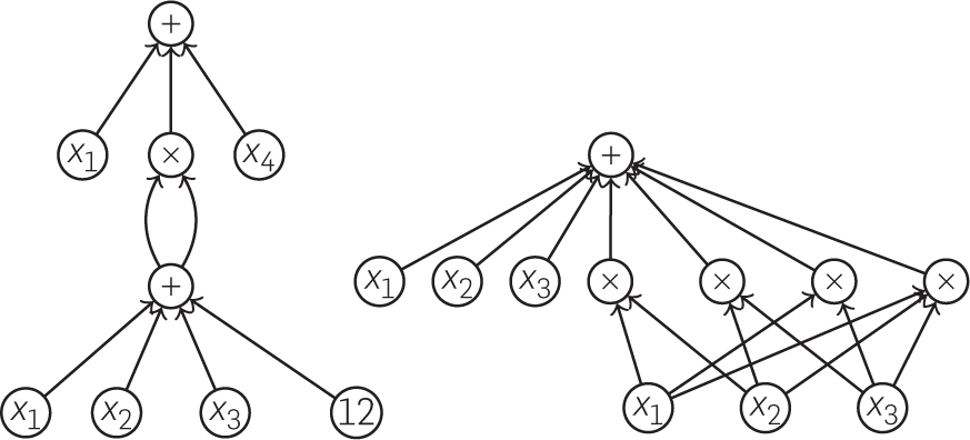
An algebraic circuit is typically visualized as a directed acyclic graph as in Figure 1 (left) where the intermediate nodes (i.e., gates) represent the basic instructions. The efficiency of the computation is captured by the size of the circuit, which is defined to be the number of edges in the underlying graph (one could also look at the number of gates, which is within a quadratic factor of the number of edges). Another parameter of efficiency is the depth of the circuit, which is the length of the longest path in the computation. The depth captures the extent to which the algorithm is parallelizable. When the underlying graph is a tree, the circuit is said to be a formula.^b

Left: an algebraic circuit. Right: a depth-2 algebraic circuit suggested by Equation (1).

Given a computational problem specified by a polynomial P, we would like to study the smallest size of an algebraic circuit (or formula) for P. In particular, there are many situations where we would like to show that a given polynomial has no small algebraic circuits. Analogous to the P vs. NP question in standard complexity theory, the principal question of this area is the Valiant’s P vs. Valiant’s NP (VP vs. VNP) question, which can equivalently be stated as the following “lower bound” question: show that the Permanent polynomial, which is a polynomial in N = n² variables of degree n has no algebraic circuits of size poly(N).

As the algebraic circuit model is required to construct the formal polynomial P under consideration, it is a syntactic model of computation, as opposed to the Boolean circuit model, which is typically only required to output the correct answer on certain inputs (e.g., Boolean inputs). As a consequence, it is intuitive that the algebraic circuit yields a more restricted family of algorithms than its Boolean variant. In particular, this implies that the problem of proving algebraic circuit lower bounds is easier than its Boolean counterpart.³ On the other hand, it is also a natural model that captures most algorithms for algebraic computational problems of the kind we care about. Resolving the VP vs. VNP question is thus seen as an important stepping stone to resolving P vs. NP.

1.2. Constant-depth circuits

What makes the VP vs. VNP question (and other similar questions in algebraic complexity) particularly alluring is that there is a very concrete strategy for resolving it based on the technique of depth-reduction. To describe this, let us start with some basic notation. A polynomial P can always be written as a sum of monomials as in Equation (1) above. Such a representation can also be visualized as a depth-2 circuit (see Figure 1 right) and is called a ΣΠ circuit for the reason that the polynomial is expressed as a sum of products of variables. Such a representation is extremely simple to analyze: for example, any polynomial P has a unique such minimal representation, the size of which is essentially the number of monomials in the polynomial. For a polynomial in N variables of degree d, this is typically around N^d.

However, things get much more interesting with just one more layer of complexity. For instance, consider ΣΠΣ circuits, which are sums of products of sums of variables. Such circuits can be much more succinct than SP. For instance, the polynomial from Equation (1) can be written more succinctly as

(1 + x_{1}) (1 + x_{2}) (1 + x_{3}) - 1,

which can be seen as a simple ΣΠΣ circuit. More generally, a surprising and beautiful result of Gupta et al.⁹ (building on many previous results¹^,¹²^,²⁴) showed that if a polynomial P on N variables of degree d has an algebraic circuit of size poly(N), then it has a ΣΠΣ circuit of size $N^{O (\sqrt{d})}$ . While this is quite large, it is still considerably smaller than the trivial N^d in the ΣΠ case. In particular, it is feasible that we could show VP is not VNP simply by showing that the Permanent (or another similar polynomial) has no ΣΠΣ circuits of this size!

In terms of depth, ΣΠΣ circuits are just depth-3 circuits. So this means that a strong enough lower bound for depth-3 circuits implies a separation between VP and VNP. No such connection between constant-depth circuit lower bounds and general circuit lower bounds is known in the non-algebraic (i.e., Boolean) setting.

In particular, the results above illustrate how useful it would be to have strong constant-depth circuit lower bounds in the algebraic setting. Unfortunately, however, these bounds have so far been difficult to demonstrate. Despite extensive work in the area, and many beautiful lower bound results against restricted models of circuits,⁸^,¹⁵^,¹⁶ even super-polynomial lower bounds against ΣΠΣ circuits have remained an open question.

In this work, we show superpolynomial lower bounds against general ΣΠΣ circuits and more generally, against circuits whose depth is a constant independent of the number of variables and the degree of the underlying polynomial. More precisely we show the following.

Theorem 1 (Main Result).

Let N, d be growing parameters with d = o(log N). There is an explicit polynomial P_N,d(x₁, …, x_N) that has no algebraic circuits of constant depth and polynomial size. More precisely, for any fixed Δ, there is a constant ε > 0 such that any circuit of depth Δ computing P_N,d has size at least $N^{Ω (d^{ε})}$ .

In the case of ΣΠΣ circuits (i.e., Δ = 3), we get a lower bound of $N^{Ω (\sqrt{d})}$ . By the result of Gupta et al.⁹ mentioned above, any asymptotic improvement in the exponent in this bound could potentially separate VP from VNP.

Moreover, the polynomial P_N,d itself is easy to describe and encodes the natural problem of Matrix Multiplication. Assume n and d are such that N = dn². The polynomial P_N,d is the Iterated Matrix Multiplication polynomial IMM_n,d on N = dn² variables, defined as follows. The underlying variables are partitioned into d sets X₁, …, X_d of size n², each of which is visualized as an n × n matrix with distinct variable entries. Then IMM_n,d is defined to be the polynomial that is the (1, 1)th entry of the product matrix X₁ · X₂ … X_d.

1.3. Consequence of polynomial identity testing

Another important question in algebraic complexity deals with the algorithmic analysis of a given algebraic circuit. More specifically, the Polynomial Identity Testing (PIT) problem is the following algorithmic problem: given an algebraic circuit C computing a polynomial P, is this polynomial a nonzero polynomial? That is, are any of the coefficients of P non-zero?

To illustrate the hardness of this question, it is worth noting that the number of potential monomials in the polynomial P is exponentially large, and hence expanding out to compute each of the coefficients of P would take exponential time. Nevertheless, it is known that there is a polynomial-time randomized algorithm for this problem. We simply evaluate P at a random point and check if P evaluates to a non-zero value at that point. The circuit representation allows for efficient evaluation of P and hence this algorithm is efficient. However, the algorithm might make an error: specifically, this happens when P is non-zero but the algorithm happens to choose a point where P evaluates to zero. However, the probability of this can be shown to be small.

The algorithmic challenge is therefore to come up with a deterministic (i.e., non-randomized) efficient algorithm for this polynomial. This problem has seen extensive work over the past couple of decades (see e.g., the surveys¹³^,²⁰^,²²), with the introduction of many specialized tools to solve restricted variants of this problem. Nevertheless, even sub-exponential time deterministic algorithms for PIT for simple classes such as ΣΠΣ circuits remained open until this work.

The difficulty of this problem is explained by the strong connections that have been made between this question and the problem of showing lower bounds against algebraic circuits. An influential result of Kabanets and Impagliazzo¹¹ showed that superpolynomial lower bounds against general algebraic circuits imply deterministic sub-exponential time algorithms for general PIT. Later results have tried to extend this algebraic hardness vs. randomness framework in several different ways.⁵^,⁶^,¹³ Specifically, Dvir et al.⁶ proved that hardness for constant-depth circuits implies a deterministic algorithm for PIT for constant-depth circuits. In a recent paper, Chou et al.⁵ refined this result and improved the dependence on the degree of the polynomial.

We observe that this result from Chou et al.⁵ combined with our lower bound from Theorem 1 gives the first sub-exponential time deterministic algorithm for PIT for algebraic circuits of any constant depth. Specifically, we get the following.

Corollary 2.

The following holds for any ε > 0. Let C be an algebraic circuit of size s ≤ poly(n) and constant depth Δ computing a polynomial on n variables. There is a deterministic algorithm that can check whether the polynomial computed by C is identically zero or not in time ${(s^{Δ + 1} \cdot n)}^{O (n^{ε})}$ .

2. The Approach: “Hardness Escalation”

While lower bounds against general algebraic circuits have been hard to prove, we do have several beautiful results against restricted kinds of algebraic circuits, such as Homogeneous, Multilinear, and Set Multilinear circuits. As these will be useful in the sequel, we review some of these definitions below.^c

Recall that a multilinear polynomial P(x₁, …, x_N) is one in which each variable x_i has degree at most 1, and a homogeneous polynomial is one that is a linear combination of monomials of the same total degree. If the underlying variable set is partitioned into d variable sets X₁, …, X_d, then P is said to be set-multilinear with respect to this variable partition if P is a linear combination of monomials that contains one variable from each variable set among X₁, …, X_d; note that a set-multilinear polynomial is both multilinear and homogeneous (of degree d). For example, the n × n Determinant is a set-multilinear polynomial w.r.t the variable partition corresponding to the rows of the underlying matrix, and the polynomial IMM_n,d defined above is set-multilinear w.r.t. the partition into matrices X₁, …, X_d.

Given a set-multilinear polynomial P (w.r.t. variable partition X₁, …, X_d), it is natural to look at algebraic circuits computing P that themselves have the same structure. In particular, an algebraic circuit is said to be set-multilinear if each internal gate computes a set-multilinear polynomial in a subset of X₁, …, X_d. Similarly, a multilinear or homogeneous circuit is one where each internal node computes a multilinear or homogeneous polynomial respectively. For each such restricted type of circuit, we have nontrivial lower bounds on the sizes of circuits computing explicit polynomials (also restricted in the same way).¹⁴^,¹⁵^,¹⁶ An important result of Nisan and Wigderson¹⁵ proved lower bounds against small-depth set-multilinear and homogeneous circuits computing IMM_n,d. Building upon this, Raz¹⁶ showed superpolynomial lower bounds on the size of any (unbounded depth) multilinear formula computing the n × n Determinant and Permanent.

It is natural to ask if we can use these lower bounds against restricted kinds of circuits to prove lower bounds against more general algebraic circuits. Such “hardness escalation” results have appeared in many areas in computational complexity, including Algebraic complexity theory. Strassen²³ and Raz¹⁷ both observed (in different settings) that lower bounds against small-depth circuits computing low-degree polynomials imply lower bounds against larger depth circuits. More recently, Raz¹⁸ showed that if a homogeneous or set-multilinear polynomial of degree d has an algebraic formula of size s, then it also has a homogeneous or set-multilinear formula of size poly(s) · (log s)^O(d) respectively. In particular, for a homogeneous (resp. set-multilinear) polynomial P of degree d = O(log N / log log N), it follows that P has a formula of size poly(N) if and only if P has a homogeneous (resp. set-multilinear) formula of size poly(N).^d

The latter result implies that if we could prove homogeneous or set-multilinear formula lower bounds of the form $N^{ω_{d} (1)}$ (i.e., the exponent goes to infinity with d) for a polynomial P with N variables and degree d, then we would have superpolynomial general algebraic formula lower bounds. In particular, this would imply lower bounds against constant-depth algebraic circuits, as any constant-depth algebraic circuit can be converted to an algebraic formula with only a polynomial blow-up.^e

Unfortunately, known results do not yield such lower bounds. In the homogeneous case, we have strong lower bounds against certain formulas of depth at most 4,¹⁴^,¹⁵ but this falls short of proving anything for general formulas as Raz’s “homogenization” result does not preserve the depth of the formula (in fact, known results for homogeneous formulas stop yielding lower bounds exactly in the regime where they would yield implications for general circuits). In the set-multilinear, and more generally multilinear case, we do have lower bounds against formulas of large depth,¹⁵^,¹⁶ but all such lower bounds are of the form f (d) · poly(N) where f (d) is a superpolynomial (and subexponential) function of d. With analogy to Parameterized Complexity Theory, we call such bounds Fixed Parameter Tractable (FPT) bounds. Our motivating question is if we can prove strong non-FPT lower bounds against restricted types of circuits or formulas in a setting where we can use them for lower bounds for general algebraic circuits or formulas. We show that this is indeed possible.

2.1. Technical results

Our main lower bound result is a strong non-FPT lower bound against constant-depth set-multilinear circuits, considerably strengthening known results in this direction.

We prove our lower bounds for the IMM_n,d polynomial on N = dn² variables as defined above. This polynomial has a simple divide-and-conquer-based set-multilinear formula of size n^{O(log d)}, and more generally for every Δ ≤ log d, a set-multilinear formula of depth 2Δ and size $n^{O ({Δ d}^{1 / Δ})}$ . It is reasonable to conjecture that this simple upper bound is tight up to the constant in the exponent for set-multilinear formulas.

This has been shown for set-multilinear, and more generally, for homogeneous circuits of depths 3 and 4.⁷^,¹⁴^,¹⁵ However, as far as we know, no superpolynomial non-FPT lower bounds were known for any depths greater than 4, even under the set-multilinearity restriction. We show such lower bounds for all constant depths.

Theorem 3 (Lower bound against set-multilinear circuits).

Assume d ≤ (log n)/100. For any constant depth Δ, any set-multilinear circuit C computing IMM_n,d of depth at most Δ must have size at least ${n^{d}}^{ε}$ , where ε is a constant that depends only on Δ. In the particular case that Δ = 5, the size of C must be at least $n^{Ω (\sqrt{d})}$ .

With these stronger non-FPT lower bounds for set-multilinear circuits in place, we are able to derive lower bounds against stronger families of algebraic circuits via hardness escalation arguments.

First, we show that any homogeneous circuit of depth Δ and size s computing a set-multilinear polynomial P of degree d can be converted to a set-multilinear circuit with the same depth for P of size s · d^O(d). Putting this together with Theorem 3, we get the first superpolynomial lower bounds (FPT or non-FPT) for homogeneous circuits of depth greater than 5.

Corollary 4 (Lower bound against homogeneous circuits).

Assume d ≤ (log n)/100. For any constant depth Δ, any homogeneous circuit C computing IMM_n,d of depth at most Δ must have size at least $n^{d^{ε}}$ , where ε is a constant that depends only on Δ. In the particular case that Δ = 5, the size of C must be at least $n^{Ω (\sqrt{d})}$ .

Note that our improved non-FPT bounds are crucial for deriving the above result from Theorem 3. The previous best lower bound of $2^{Ω (\sqrt{d})}$ due to Nisan and Wigderson¹⁵ does not suffice for this, because of the d^O(d) blow-up involved in converting a homogeneous circuit to one that is set-multilinear.

Next, we show that any (possibly non-homogeneous) algebraic circuit of depth Δ and size s computing a homogeneous polynomial P of degree d can be converted to a homogeneous circuit for P of depth 2Δ + 1 and size $2^{O (\sqrt{d})}$ . This implies the main result Theorem 1.

3. An Illustration: Depth-3 Circuits

We prove in this section the case Δ = 5 of Theorem 3 and Corollary 4 and the case Δ = 3 of Theorem 1.

3.1. Reduction to set-multilinear depth 5

In the next sub-section, we will show super polynomial lower bounds for small-degree polynomials against set-multilinear formulas of some constant depth. We want to extend these lower bounds to the general setting (i.e., without the set-multilinearity constraint).

Raz¹⁸ showed that if there is a fanin-2 formula of size s and depth Δ that computes a set-multilinear polynomial over the disjoint sets (X₁, …, X_d), then there exists also a fanin-2 set-multilinear formula of size $O ((Δ + 2)^{d} s)$ and depth Δ that computes the same polynomial. However, the fanin-2 constraint is an issue when we want to deal with constant-depth circuits.

We show here that we can get a similar result for circuits with arbitrary fanins at the cost of a size blow-up of d^O(d) poly(s) and an increase of the depth by a factor of at most 2.

Proposition 5.

Let s, N, d be growing parameters with s ≥ Nd. If C is a circuit of size at most s and depth at most 3 computing a set-multilinear polynomial P over the sets of variables (X₁, …, X_d) (with |X_i| ≤ N), then there is a set-multilinear circuit $\tilde{C}$ of size d^O(d)poly(s) and depth at most 5 computing P.

Similar to Raz’s approach, we start by homogenizing the circuit and then we set-multilinearize it. In particular, the previous proposition is just the composition of Lemmas 6 and 7.

Non-homogeneous to homogeneous circuits.

It was already noticed⁹^,¹⁰ that we can convert nonhomogeneous formulas of depth 3 to homogeneous formulas of depth 5 with a relatively small size blow-up.

Indeed, a general ΣΠΣ circuit of size s yields a formula of the following kind

F = Σ_{i = 1}^{s} Π_{j = 1}^{s} ℓ_{i, j}

where each l_i,j is an affine linear polynomial in the underlying variables. Note that the individual summands of the expression may compute polynomials of degree s, which is possibly much larger than d. The main observation is that, assuming that the underlying field 𝔽 has characteristic 0 (which is the case here since we chose 𝔽 = ℂ), the homogeneous degree-d part of each summand can be computed by a homogeneous formula of size poly(s) · $\exp ((O \sqrt{d}))$ . Replacing each of these terms with such a formula, we see that the same polynomial can also be computed by a homogeneous ΣΠΣΠΣ formula of size size poly(s) · $\exp ((O \sqrt{d}))$ .^f

The main observation is also easy to prove. Consider any summand T_i = l_i,1 … l_i,s. It suffices to prove the observation in the case that each l_i,j has a non-zero constant term c_j (it is easy to reduce to this case). In this case, we can write

Γ_{i} = (Π_{j = 1}^{s} c_{i}) \cdot Π_{j = 1}^{s} (1 + ℓ_{i, j}^{'})

where each $ℓ_{i, j}^{'}$ is a homogeneous linear polynomial. It then follows that the degree-d homogeneous part T_i,d of T_i can be written as a linear projection applied to the Elementary Symmetric Polynomial $E_{s}^{d}$ of degree d in s variables. More precisely, we have

T_{i, d} = (Π_{i = 1}^{s} c_{i}) \cdot E_{s}^{d} (ℓ_{i, 1}^{'}, …, ℓ_{i, s}^{'}) .

Shpilka and Wigderson²¹ [Theorem 5.3] proved that, over fields of characteristic 0 the polynomial $E_{s}^{d}$ has a homogeneous ΣΠΣΠ circuit of size poly(s) · $\exp (O (\sqrt{d}))$ . The result seems to be also proved independently in Hrubeš and Yehudayoff.¹⁰ Using this with the above expression, we get the following result.

Lemma 6 (Lemma 5.6 in the journal version)⁹.

Let s, N, d be growing parameters. Fix any ΣΠΣ circuit F of size at most s computing a homogeneous polynomial P(x₁, …, x_N) of degree d. Then, P can also be computed by a homogeneous ΣΠΣΠΣ circuit F′ of size at most size poly(s) $\exp (O (\sqrt{d}))$ .

Homogeneous to set-multilinear circuits.

Then we need to convert homogeneous circuits into set-multilinear ones without increasing the depth and with a relatively small size blow-up. In fact, this transformation is not really more complicated in the case of an arbitrary depth. Thus, we place ourselves here directly in this case.

Lemma 7.

Let Δ be an odd integer. Let s, N, d be growing parameters with s ≥ Nd. If C is a homogeneous circuit of size at most s and depth at most Δ computing a set-multilinear polynomial P over the sets of variables (X₁, …, X_d) (with |X_i| ≤ N), then there is a set-multilinear circuit $\tilde{C}$ of size at most (d!)s and depth at most Δ computing P.

Proof. Let us describe our new circuit $\tilde{C}$ . For any gate α of degree d_α from C, we create $d_{α}^{d}$ gates α_S in $\tilde{C}$ (we index these gates by the subsets S⊆[d] such that |S| = d_α). Now we want to link these gates such that for every gate α in C and any S⊆[d] with |S| = d_α, the depth of α_S is the same as the one of α and the polynomial computed by α_S is the projection of the polynomial computed by α to the set-multilinear part associated with S:

α_{S} = \underset{m set-multilinear over {(X_{i})}_{i \in s}}{Σ} ([m] α) m

where ([m]α) is the coefficient of the monomial m in α.

Let us do it by induction on the structure of the graph.

If α is a leaf, it is labeled either by a constant or by a variable. When d_α = 0, there is nothing to change. Otherwise d_α = 1. In C the leaf α is labeled by a variable x which belongs to X_i. We just need to label the gates by α_{i} = x and α_{j} = 0 for j ≠ i.^g

If α = c¹α¹ + … + α^pα^p is a sum gate (where the cⁱ are constants in ℂ), we just need to compute the linear combination part by part. For any S⊆[d] with |S| = d_α:

α_{S} = c^{1} α_{S}^{1} + … + c^{p} α_{S}^{p} .

Finally, if α = α¹ · … · α^p is a product gate, we need to extract all the decompositions. Let S⊆[d] with |S| = d_α:

α_{S} = \underset{(S_{1}, …, S_{p}) partition of S with \forall i, | S_{i} | = d_{α^{i}}}{Σ} α_{S_{1}}^{1} + \cdot … \cdot + α_{S_{p}}^{p} .

The size of the sum is $(\begin{matrix} d_{α} \\ d_{α^{1}}, …, d_{α^{p}} \end{matrix})$ .

Hence each leaf and sum gate α in C creates $(d_{α}^{d}) \leq d!$ new gates in $\tilde{C}$ . Each multiplication gate α in C creates $(d_{α}^{d}) \leq d!$ sum gates and $(\begin{matrix} d \\ d_{α} \end{matrix}) (\begin{matrix} d_{α} \\ d_{α^{1}}, …, d_{α^{p}} \end{matrix}) \leq d!$ new product gates. So the number of gates of $\tilde{C}$ is bounded by 2d! times the number of gates of C. Notice that we can avoid factor 2 since we do not need to keep the sum gates which come from a product gate, we can merge them with the sum gates of the next layer of the circuit. (We always assume that the output gate is a sum gate, and so there is always a next layer to merge with.) Furthermore, the depth of the gate α_S in $\tilde{C}$ is the same as the one of the gate α in C.

3.2. Lower bounds against set-multilinear depth 5

By Proposition 5, it is sufficient to get a sufficiently large lower bound against set-multilinear depth-5 circuits to prove Theorem 1 for depth-3 circuits.

In this section, we will prove the following non-FPT lower bound against set-multilinear depth-5 circuits.

Lemma 8.

Let n, d ∈(N){0} with $n \geq 4^{\sqrt{d} + 1}$ . Any set-multilinear circuit C of depth 5 computing IMM_n,d has size at least $n^{Ω (\sqrt{d})}$ .

Notice that if d ≤ (log n)/100, then the hypothesis of this lemma is immediately satisfied. Consequently, this lemma directly implies the case Δ = 5 of Theorem 3.

In the case where Δ = 3 in Theorem 1 using Proposition 5, we can transform circuit C into a depth-5 set-multilinear one of size at most d^O(d)poly(s). By Lemma 8, it implies that $d^{O (d)} poly (s) \geq n^{Ω (\sqrt{d})}$ . By the assumption d ≤ (log n)/100, we get the desired lower bound for s.

The case Δ = 5 of Corollary 4 is proved identically by replacing Proposition 5 with Lemma 7.

Therefore, all we have to do is prove Lemma 8. The proof technique is very standard: we will focus on the complexity measure of partial derivatives (introduced by Nisan and Wigderson¹⁵) and show that particular polynomials computed by small set-multilinear circuits of depth 5 have small measures. The novelty here is that we will focus on polynomials which are lopsided, that is, that are based on a partition of the variables where different parts have different sizes. It is thanks to this point that we are able to obtain new lower bounds.

The complexity measure.

So let us start by introducing the measure.

We will consider the set of words on an alphabet A⊆ℕ{0}. Let w = (w₁, …, w_d)∈ A^d For a subset S⊆[d], let w_S denote ∑_i∈S w_i. We say is w ∈ A^d b-unbiased if |w_[t]|≤b for every t ≤ d. We define $P_{w} = {i | w_{i} > 0}$ and $N_{w} = {i | w_{i} < 0}$ that is, the positive and negative indices of w respectively.

Given w, we denote by $\bar{X} (w)$ a tuple of d sets of variables (X(w₁), …, X(w_d) ) where $| X (w_{i}) | = 2^{| w_{i} |}$ . We denote by 픽_sm[𝒯] the set of set-multilinear polynomials over the tuple of sets of variables 𝒯.

Let $M_{w}^{P}$ and $M_{w}^{N}$ denote the sets of the set-multilinear monomials over only the positive and only the negative variable sets. Let $f \in F_{sm} [\bar{X} (w)]$ we define M_w(f) as the matrix of size $| M_{w}^{P} | \times | M_{w}^{N} |$ , where the rows are indexed by $M_{w}^{P}$ and the columns by $M_{w}^{N}$ and where the coefficient at the entry (m₁, m₂) is the coefficient of the monomial m₁m₂ in f.

We associate with the space $F_{sm} [\bar{X} (w)]$ the standard rank-based complexity measure relrk_w (short for “relative rank”) defined as follows. Let $f \in F_{sm} [\bar{X} (w)]$ and define

[r e l r k_{w} (f) = \frac{r a n k (M_{w} (f))}{\sqrt{| M_{w}^{P} | | M_{w}^{N} |}} = \frac{r a n k (M_{w} (f))}{2^{\frac{1}{2} Σ_{i \in [d]} | w_{i} |}} .

Intuitively, as we will want to play on the size of the subsets of variables and thus modify the maximum rank that the polynomial can have, using the relative rank rather than the usual rank allows us to more easily take into account the distance we are from the maximum rank.

We use the following properties of relrk_w.

Claim 9.

(Imbalance) Say $f \in F_{s m} [\bar{X} (w)]$ Then, ${relrk}_{w} (f) {\leq 2}^{- | w_{[d]} | / 2}$ .
(Sub-additivity) Say $f, g \in F_{s m} [\bar{X} (w)]$ . Then relrk_w(f + g) ≤ relrk_w(f) + relrk_w(g).
(Multiplicativity) Say f = f₁ · f₂·…· f_t and assume that for each $i \in [t], f_{i} \in F_{s m} [\bar{X} (w_{| S_{i}})]$ where (S₁, …, S_t) is a partition of [d] and for each $i \in [t], w_{| S_{i}}$ stands for the sub-word of w indexed by S_i. Then $r e l r k_{w} (f) = r e l r k_{w} (f_{1} \cdot f_{2} \cdot … \cdot f_{t}) = \underset{i \in [t]}{Π} r e l r k_{w_{| s_{i}}} (f_{i}) .$

Proof. We have that $| M_{w}^{P} | = 2^{Σ_{i \in {P_{w}}^{w_{i}}}}$ and $| M_{w}^{N} | = 2^{- Σ_{i \in {N_{w}}^{w_{i}}}}$ . So $2^{| w_{d} |}$ is just the ratio of the larger dimension of M_w(f) by the smaller one. As the rank of a matrix is bounded by the minimum between its number of rows and its number of columns, it implies the first inequality of the claim.

The subadditivity property directly follows from the facts that M_w(f + g) = M_w(f) + M_w(g) and that the rank of a matrix is subadditive.

The multiplicative argument is standard too. As the product is set-multilinear, it implies that the matrix M_w(f₁ · … · f_t) is the matrix M_w(f₁)⊗…⊗M_w(f_t) where the symbol ⊗ stands for the Kronecker product. Finally, the rank is known to be multiplicative with respect to the Kronecker product. So,

\begin{matrix} r e l r k_{w} (f_{1} \cdot f_{2} \cdot … \cdot f_{t}) = \frac{r a n k (M_{w} (f_{1} \cdot … \cdot f_{t}))}{{2^{\frac{1}{2} \sum_{j \in [d]}}}^{| w_{j} |}} \\ = \underset{i \in [t]}{Π} \frac{r a n k (M_{w} (f_{i}))}{2^{\frac{1}{2} {\sum_{j \in s_{i}}}^{| w_{j}}}} = \underset{i \in [t]}{Π} r e l r k_{w_{| S_{i}}} (f_{i}) . \end{matrix}

Word polynomials and iterated matrix multiplication polynomial.

We said we will prove lower bounds for lopsided polynomials. Unfortunately, all variables parts of the polynomial IMM_n,d have the same size (which is n²). In fact, we will prove the lower bound for the word polynomial which is a “set-multilinear” projection of IMM_n,d (The projection is called set-multilinear because it preserves the set-multilinearity). So let us define this polynomial.

Let w ∈ A^d be any word. For any such word, we define a polynomial P_w. Say $\bar{X} (w) = (X_{1}, …, X_{d})$ and since each X_i has size $2^{| w_{i} |}$ , we assume that the variables of X_i are labeled by strings in ${0, 1}^{| w_{i} |}$ .

Given any monomial $m \in F_{sm} [\bar{X} (w)]$ let m₊ denote the corresponding “positive” monomial from $M_{w}^{P^{+}}$ and m₋ the corresponding “negative” monomial from $M_{w}^{N}$ . As each variable of $\bar{X} (w)$ is labeled by a Boolean string and each set-multilinear monomial over any subset of $\bar{X} (w)$ is associated with a string of variables, we can associate any such monomial m′ with a Boolean string σ(m′). More precisely, if j₁ < … < j_t and $m' = x_{σ_{1}}^{(j_{1})} x_{σ_{2}}^{(j_{2})} … x_{σ_{t}}^{(j_{t})}$ with $x_{σ_{i}}^{(j_{i})} \in X_{j_{i}}$ and $σ_{i} \in {0, 1}^{| w_{j_{i}} |}$ for each i∈[t], then σ(m′) is defined to be σ₁…σ_t. If w is b-unbiased, the difference of length of the strings σ(m₊) and σ(m₋) is at most b. We will write σ(m₊) ~ σ(m₋) when the shorter one is a prefix of the other one.

The polynomial P_w is defined as follows:

P_{w} = \underset{m \in F [\bar{X} (w)], σ (m_{+}) ~ σ (m_{-})}{Σ} m .

Clearly, the matrices M_w(P_w) are full-rank (i.e., have a rank equal to either the number of rows or the number of columns, whichever is smaller). So, ${relrk}_{w} (P_{w}) = 2^{- | w_{[d]} | / 2} \geq 2^{- b / 2}$ .

We observe that P_w can be obtained as a set-multilinear restriction of IMM_n,d for an appropriate choice of n. Formally, one can show the following. The proof is straightforward but omitted from this extended abstract.

Lemma 10.

Let w ∈ A^d be any word which is b-unbiased. If there is a set-multilinear circuit computing ${IMM}_{2^{b}, d}$ of size s and depth Δ, then there is also a set-multilinear circuit of size s and depth Δ computing a polynomial $P_{w} \in F_{s m} [\bar{X} (w)]$ such that relrk_w(P_w) ≥ 2^−b/2.

Proof of Lemma 8.

We now have all the ingredients to tackle the proof of the lemma.

It is a standard fact that any circuit of constant depth can be converted to a formula with only a polynomial blow-up. So it suffices to show the following.

Claim 11.

Let d ≥ 16 and $k > 2 \sqrt{d}$ be an integer. Let w be any word of length d on the alphabet ${- k, ⌊ k - k / \sqrt{d} ⌋}$ . Then any set-multilinear formula C of depth 5 and of size s satisfies

$[r e l r k_{w} (C) \leq s \cdot 2^{- \frac{k \sqrt{d}}{8}} .$

Indeed, by fixing $k = ⌊ \log_{2} n ⌋$ we have $k > 2 \sqrt{d}$ . We can construct by induction a word w on the alphabet ${- k, ⌊ k - k / \sqrt{d} ⌋}$ which is k-unbiased. Indeed, if |w_[i]| ≤ 0, we choose $w_{i + 1} = ⌊ k - k / \sqrt{d} ⌋$ , otherwise we set w_i+1 = −k. By Lemma 10 and Claim 11, we get the lower bound:

\begin{matrix} s \geq 2 \frac{k \sqrt{d}}{8} 2^{- k} \geq 2^{(\log_{2} n - 1) \frac{\sqrt{d}}{8} - \log_{2} n} \\ \geq n^{\frac{\sqrt{d}}{8}} 2^{- \frac{\log_{2} n}{l 6} - \log_{2} n} \geq n^{\frac{\sqrt{d}}{8} - \frac{17}{16}} \end{matrix}

for the polynomial ${IMM}_{2^{k}, d}$ against set-multilinear circuits of depth 5.

Proof of Claim 11. We know C is a depth 5 formula, so we can define C = C₁ + … + C_t where each C_i is of the form ΠΣΠΣ and has size s_i. We say that C_i is of type 1 if some factor of C_i has degree $\geq \sqrt{d} / 2$ , otherwise it is of type 2.

If C_i is of type 1, then $C_{i} = C_{i, 1} \cdot … \cdot C_{i, t_{i}}$ . Up to reordering, we can assume that C_i,1 is a sum of products of linear forms of degree at least $\sqrt{d} / 2$ . Notice that if L is a linear form on variables X(w_i), we have $relrk (L) \leq 2^{- | w_{i} | / 2} \leq 2^{- (k - k / \sqrt{d} - 2) / 2}$ . In particular, by the multiplicativity and sub-additivity of relrk_w (Claim 9), $\begin{matrix} r e l r k_{w} (C_{j}) \leq r e l r k_{w} (C_{i, 1}) \leq s_{i} 2^{- \frac{k \sqrt{d} - k - \sqrt{d}}{2 \sqrt{d}} \deg (C_{i}, 1)} \\ \leq s_{j} 2 \frac{k \sqrt{d} - k - \sqrt{d}}{4} \leq s_{j} 2^{- \frac{k \sqrt{d}}{8}} . \end{matrix}$
If C_i is of type 2, then $C_{i} = C_{i, 1} \cdot … \cdot C_{{i, t}_{i}}$ where each factor C_ij has degree $< \sqrt{d} / 2$ . Each C_ij is a set-multilinear formula over a subset (X(w_p): p∈S_j) for some S_j ⊆[d] where $S_{1}, …, S_{t_{i}}$ partition [d]. Let $w^{i 1}, … w^{{i t}_{i}}$ be the corresponding decomposition of w. That is, $w^{i j} = w_{{| S}_{j}}$ . Recall that for a word w^ij we defined in the preliminaries $w_{S_{j}}^{i j}$ as the sum of its entries.
Let j∈[t_i]. Let a_ij be the number of positive indices in w^ij. If 2a_ij ≤ deg(C_i,j), then
$w_{S_{j}}^{i j} \leq - \frac{k}{2 \sqrt{d}} \deg (C_{i, j}) .$
Otherwise, we have
$\begin{matrix} | w_{S_{j}}^{i j} | = | a_{i j} ⌊ k - \frac{k}{\sqrt{d}} ⌋ - (\deg (C_{i, j}) - a_{j j}) k | \\ = | a_{j j} k - a_{i j} ⌈ \frac{k}{\sqrt{d}} ⌉ - \deg (C_{i, j}) k + a_{i j} k | \\ > (2 a_{i j} - \deg (C_{i j}) - \frac{a_{j j}}{\sqrt{d}}) k - a_{i j} \\ > \frac{k}{2} - \frac{k}{4} = \frac{k}{2} \cdot \frac{1}{2} \\ > \frac{k \deg (C_{i, j})}{2 \sqrt{d}} . \end{matrix}$
So in both cases, $| W_{S_{j}}^{i_{j}} | \geq \frac{k \deg (C_{i, j})}{2 \sqrt{d}}$ .
In particular, $r e l r k_{w} (C_{i}) \leq Π_{j = 1}^{t_{i}} 2^{- \frac{1}{2} | w_{S_{j}}^{i j} |} \leq 2^{\frac{k d}{4 \sqrt{d}}} \leq s_{i} 2^{- \frac{k \sqrt{d}}{8}} .$

The result of the claim directly follows from the subadditivity of the measure.

4. What Happens for Larger Constant Depths

To prove Theorem 1, Theorem 3, and Corollary 4 in their generality (i.e., for any constant depths), we generalize the depth-3 approach detailed above. To do that, we just need to generalize Proposition 5 and Lemma 8 for a larger depth. We will just sketch here the ideas to obtain such a generalization. The detailed proof of the main theorem can be found in the full version of this paper.

4.1. The set-multilinearization transformation

As already noticed the set-multilinearization from homogeneous circuits transformation (Lemma 7) still works for large depths. The only point there is to generalize Lemma 6 to a larger depth. Unlike the case of depth-3, this homogenization step was not known before this work. Now, inputs of a product can have now polynomials of any degree. The idea is to consider now some weighted versions of the elementary symmetric polynomials to take care of these degrees. The main difficulty now is to check that the Newton identities (which play a key role in the proof of Lemma 6) still hold in this weighted setting. But finally, we can obtain the following homogeneization result.

Lemma 12.

Let Δ be an odd integer. Let s, N, d be growing parameters with s ≥ N. If C is a circuit of size at most s and depth at most Δ computing a homogeneous polynomial P(x₁, …, x_N) of degree d, then, P can also be computed by a homogeneous circuit $\tilde{C}$ of size at most poly(s) $2^{O (\sqrt{d})}$ and depth at most 2Δ − 1.

4.2. Lower bounds for set-multilinear circuits

Then, we follow a similar path to obtain lower bounds on the size of set-multilinear circuits of any constant depth computing lopsided polynomials. In particular, we still consider the partial derivative measure. The idea now is to refine the alphabet which is used (taking values which depend on the depth Δ) so that the case where C_i is of type 2 in the proof can be tackled. Then the first case (C_i is of type 1) will correspond to an induction step.

Putting these steps in a more precise way, we can obtain the following generalization of Proposition 5 and so obtain a complete proof of Theorem 1.

Lemma 13.

Let Δ be an odd integer and let Γ = (Δ − 1)/2. Let n, d, Δ ∈ ℕ{0} with n ≥ 2^10d+1. Any set-multilinear circuit C of depth Δ computing IMM_n,d has size at least

$n^{Ω (\frac{d^{1 / (2^{Γ} - 1)}}{Γ})} .$

Acknowledgments

The authors are grateful to R. Saptharishi for spending time to discuss the proof with us. Nutan Limaye was partially funded by SERB project File no. MTR/2017/000909. Sébastien Tavenas was funded by the project BIRCA from the IDEX of Univ. Grenoble Alpes (Contract 183459). He also benefited from accommodation paid by IIT Bombay during a visit of the other two authors.

Submit an Article to CACM

CACM welcomes unsolicited submissions on topics of relevance and value to the computing community.

You Just Read

Superpolynomial Lower Bounds Against Low-Depth Algebraic Circuits

View in the ACM Digital Library

DOI

10.1145/3611094

February 2024 Issue

Vol. 67 No. 2

Pages: 101-108

Table of Contents

Join the Discussion (0)

Become a Member or Sign In to Post a Comment

The Latest from CACM

Explore More

BLOG@CACM Apr 29 2024

A Brief History of Embodied Artificial Intelligence, and Its Future Outlook

Shaoshan Liu and Shuang Wu

Architecture and Hardware

Credit: Getty Images Figure floating amidst vertical beams of light, illustration

BLOG@CACM Apr 26 2024

Optimizing Energy Efficiency in Datacenters with Advanced Cooling Technologies

Alex Williams

Architecture and Hardware

Credit: Getty Images Servers in snowy setting.

News Apr 23 2024

Maximizing Power Grid Security

R. Colin Johnson

Security and Privacy

Shape the Future of Computing

ACM encourages its members to take a direct hand in shaping the future of the association. There are more ways than ever to get involved.

Get Involved

Communications of the ACM (CACM) is now a fully Open Access publication.

By opening CACM to the world, we hope to increase engagement among the broader computer science community and encourage non-members to discover the rich resources ACM has to offer.

Learn More

Abstract

1. Introduction

1.1. Algebraic complexity

1.2. Constant-depth circuits

1.3. Consequence of polynomial identity testing

2. The Approach: “Hardness Escalation”

2.1. Technical results

3. An Illustration: Depth-3 Circuits

3.1. Reduction to set-multilinear depth 5

Non-homogeneous to homogeneous circuits.

Homogeneous to set-multilinear circuits.

3.2. Lower bounds against set-multilinear depth 5

The complexity measure.

Word polynomials and iterated matrix multiplication polynomial.

Proof of Lemma 8.

4. What Happens for Larger Constant Depths

4.1. The set-multilinearization transformation

4.2. Lower bounds for set-multilinear circuits

Acknowledgments

Superpolynomial Lower Bounds Against Low-Depth Algebraic Circuits

DOI

February 2024 Issue

Related Reading

Join the Discussion (0)

Become a Member or Sign In to Post a Comment

Shape the Future of Computing

Communications of the ACM (CACM) is now a fully Open Access publication.