Abstract
We present an algorithm that computes exact maximum flows and minimum-cost flows on directed graphs with m edges and polynomially bounded integral demands, costs, and capacities in m1+o(1) time. Our algorithm builds the flow through a sequence of m1+o(1) approximate undirected minimum-ratio cycles, each of which is computed and processed in amortized mo(1) time using a new dynamic graph data structure.
Our framework extends to algorithms running in m1+o(1) time for computing flows that minimize general edge-separable convex functions to high accuracy. This gives almost-linear time algorithms for several problems including entropy-regularized optimal transport, matrix scaling, p-norm flows, and p-norm isotonic regression on arbitrary directed acyclic graphs.
1. Introduction
The maximum flow problem and its generalization, the minimum-cost flow problem, are classic combinatorial graph problems that find numerous applications in engineering and scientific computing. These problems have been studied extensively over the last seven decades, starting from the work of Dantzig and Ford-Fulkerson. Several important algorithmic problems can be reduced to minimum-cost flows, for example, max-weight bipartite matching, min-cut, and Gomory-Hu trees. The origin of numerous significant algorithmic developments such as the simplex method, graph sparsification, and link-cut trees can be traced back to seeking faster algorithms for maximum flow and minimum-cost flow.
1.1. Problem formulation
Formally, we are given a directed graph G = (V, E) with |V| = n vertices and |E| = m edges, upper/lower edge capacities u+, u− ∈ ℝE, edge costs c ∈ ℝE, and vertex demands d ∈ ℝV with ∑v∈V dv = 0. Our goal is to solve the following linear program for the minimum-cost flow problem
(1)where the last constraint, B⊤ f = d, succinctly captures the requirement that the flow f satisfies vertex demands d, where B ∈ℝE×V is the edge-vertex incidence matrix defined as B((a,b),v) is 1 if v = a, −1 if v = b, and 0 otherwise.
In this extended abstract, we assume that all and dv are integral and polynomially bounded in n since this paper focuses on weakly-polynomial algorithms for the maximum flow and minimum-cost flow problems.
1.2. Previous work
There has been extensive work on maximum flow and minimum-cost flow. Here, we briefly discuss some highlights from this work to help place our work in context.
Starting with the first pseudo-polynomial time algorithm by Dantzig14 for maximum-flow that ran in O(mn2U) time where U denotes the maximum absolute capacity, approaches to designing faster flow algorithms were primarily combinatorial, working with various adaptations of augmenting paths, cycle canceling, blocking flows, and capacity/cost scaling. A long line of work led to a running time of Õ(m min{m½, n⅔})15, 18,19,21 for maximum flow, and Õ(mn)17 for minimum-cost flow. These bounds stood for decades.
In a breakthrough work on solving Laplacian linear systems and computing electrical flows, Spielman and Teng34 introduced a novel set of ideas and tools for solving flow problems using combinatorial techniques in conjunction with continuous optimization methods. To deploy these methods, flow algorithms researchers have used graph-algorithmic techniques to solve increasingly difficult subproblems that drive powerful continuous methods.
In the context of maximum flow and minimum-cost flow, Daitch and Spielman13 demonstrated the power of this paradigm by using a path-following interior point method (IPM) to reduce the minimum-cost flow problem to solving a sequence of roughly electrical flow (ℓ2) problems. Since each of these ℓ2 problems could then be solved in nearly-linear time using the fast Laplacian solver by Spielman-Teng, they achieved an Õ(m1.5) time algorithm for minimum-cost flow, the first progress in two decades. They showed that a key advantage of IPMs is that they reduce flow problems on directed graphs to flow problems on undirected graphs, which are easier to work with.
While other continuous optimization methods have been used in the context of maximum flow, even leading to nearly-linear time (1+ɛ)-approximate undirected maximum flow and multicommodity flow algorithms,12,23,30,32,33 to date all approaches for exact maximum flow and minimum-cost flow rely on the framework suggested by Daitch and Spielman of using a path-following IPM to reduce to a small but polynomial number of convex optimization problems. Notable achievements include an m4/3+o(1)U1/3 time algorithm for bipartite matching and unit-capacity maximum flow.4,22,27,28,29 Further, for general capacities, minimum-cost flow algorithms were given with runtimes Õ(m + n1.5)8,9,10 and Õ(m3/2–1/58).5,6,16,35 In both of these results, the development of efficient data structures to solve the sequence of ℓ2 sub-problems in amortized time sub-linear in m has played a key role in obtaining these runtimes. Yet, despite this progress, the best running time bounds remain far from linear.
1.3. Our result
We give the first almost-linear time algorithm for minimum-cost flow, achieving the optimal running time up to subpolynomial factors.
There is an algorithm that, on a graph G = (V, E) with m edges, vertex demands, upper/lower edge capacities, and edge costs, all integral with capacities and costs bounded by a polynomial in n, computes an exact minimum-cost flow in m1+o(1) time with high probability.
Our algorithm can be extended to work with capacities and costs that are not polynomially bounded at the cost of an additional logarithmic dependency in both the maximum absolute capacity and the maximum absolute cost.
We make two key contributions to achieve our result. First, we develop a novel potential-reduction IPM, similar to Karmarkar’s original work.20 Our IPM is worse in some ways than existing path-following IPMs because it needs more updates to converge to a good solution. However, our new IPM reduces the minimum-cost flow problem to a sequence of update subproblems that have a more combinatorial structure than those studied before. This enables our second key contribution, a data structure that solves our sequence of update subproblems extremely quickly.
In addition to the use of highly combinatorial updates, our new IPM has three crucial properties. The IPM is (a) robust to approximation error in subproblems, (b) stable in terms of the subproblems it defines, and (c) stable in terms of a good solution to the subproblems. These features allow us to solve the sequence of update subproblems much faster by developing a powerful data structure, yielding a much faster algorithm overall. Thus, instead of making graph algorithms more suitable for continuous optimization, we made continuous optimization more suitable for graph algorithms.
We call the update subproblem that our IPM yields min-ratio cycle: This problem is specified by a graph where every edge has a “gradient” and a “length.” The problem asks us to find a cycle that minimizes the sum of (signed, directed) edge gradients relative to its (undirected) length.
Our data structure for solving the sequence of min-ratio cycle problems is our second key contribution. As a first observation, we show that if we sample a random “low-stretch” spanning tree of the graph, then with constant probability, some fundamental tree cycle approximately solves the min-ratio cycle problem. Recall a fundamental tree cycle is a cycle defined by a single non-tree edge and the unique tree path between its endpoints. Unfortunately, this simple approach fails after a single flow update, as the IPM requires us to change the gradients and lengths after each update.
To maintain a set of trees that repeatedly allow us to identify good update cycles, we develop a hierarchical construction based on a recursive approach. This requires us to repeatedly construct and contract a random forest (which partially defines our tree), and then recurse on the resulting smaller graph, which we call a core graph. Furthermore, to enable recursion, we need to reduce the edge count in the core graph. We achieve this using a new spanner construction, which identifies a sparse subgraph of the core graph on which to recurse and detects if the removed edges damage the min-ratio cycle. Maintaining the core graphs and spanners in our recursive construction requires us to develop an array of novel dynamic graph techniques, which may be of independent interest.
1.4. Applications
Our result in Theorem 1.1 has a wide range of applications. By standard reductions, it gives the first m1+o(1) time algorithms for bipartite matching, worker assignment, negative-lengths single-source shortest paths, and several other problems. For the negative-lengths shortest path problem, Bernstein, Nanongkai, and Wulff-Nilsen obtained the first m · poly(log m) time algorithm in an independent and concurrent work.7
Using recent reductions from various connectivity problems to maximum flow, we also obtain the first m1+o(1) time algorithms to compute vertex connectivity and Gomory-Hu trees in undirected, unweighted graphs,1,25 and (1 + ɛ)-approximate Gomory-Hu trees in undirected weighted graphs.26 We also obtain the current fastest algorithm to find the global min-cut in a directed graph.11 Finally, we obtain the first almost-linear-time algorithm to compute the approximate sparsest cuts in directed graphs.
Additionally, our algorithm extends to computing flows that minimize general edge-separable convex objectives.
Consider a graph G with demands d, and an edge-separable convex cost function cost(f) = ∑e coste (fe) for “computationally efficient” edge costs coste. Then in m1+o(1) time, we can compute a (fractional) flow f that routes demands d and cost(f) ≤ cost(f⋆)+exp(−logC m) for any constant C > 0, where f⋆ minimizes cost(f⋆) over flows with demands d.
This generalization gives the first almost-linear-time algorithms for solving entropy-regularized optimal transport (equivalently, matrix scaling), p-norm flow problems, and p-norm isotonic regression for p∈[1,∞].
2. Overview
2.1. Computing minimum-cost flows via undirected min-ratio cycles
Recall the linear program for minimum-cost flow given in Equation (1). We assume that this LP has a unique optimal solution at f⋆ ∈ ℝE and let F⋆ = c⊤ f⋆ (this can be achieved by a negligible perturbation using the famous Isolation Lemma).
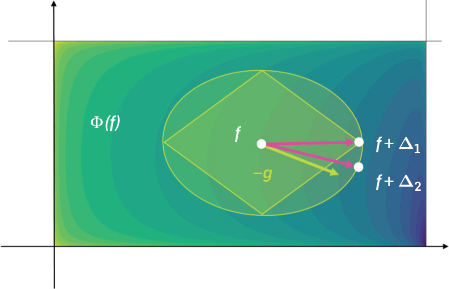
For our algorithm, we use a potential-reduction interior point method,20 where in each iteration we measure progress by reducing the value of the potential function
for α = 1/(1000 log mU). The reader can think of the barrier x−α as the more standard −log x for simplicity instead. We use it for technical reasons beyond the scope of this paper.
Using standard techniques, one can add O(n) additional, artificial edges of large capacity and cost to the graph G such that the optimal solution to the minimum-cost flow problem remains unchanged (and in particular is not supported on the artificial edges) and such that one can easily find a feasible flow f on the artificial edges such that B⊤ f = d with bounded potential, that is, Φ(f) = O(m log m).
Given the current feasible solution f, the potential reduction interior point method asks to find a circulation Δ, that is, a flow that satisfies B⊤ Δ = 0, such that Φ(f + Δ) ≤ Φ(f) − m−o(1). Given Δ, it then sets f ← f + Δ and repeats. When Φ(f) ≤ −200m log mU, we can terminate because then c⊤ f − F⋆ ≤ (mU)−10, at which point standard techniques let us round to an exact optimal flow.13 Thus if we can reduce the potential by m−o(1) per iteration, the method terminates in m1+o(1) iterations.
Let us next describe how to find a circulation Δ that reduces the potential sufficiently. Given the current flow f, defining the gradient and lengths and , and we let be the matrix with these lengths on the diagonal and zeros elsewhere. We can then define the min-ratio cycle problem
(2)Given any solution Δ to this problem with g(f)⊤ Δ/∥LΔ∥1≤−κ for some κ < 1/100, scaled so that ∥LΔ∥1 = κ/50. Then a direct Taylor expansion shows that Φ(f + Δ) ≤ Φ(f) − κ2/500. Hence, it suffices to show that such a Δ exists with , because then a data structure that returns an mo(1)-approximate solution still has κ = m−o(1), which suffices. Fortunately, the witness circulation Δ(f⋆) = f⋆ − f satisfies .
We emphasize that it is essential for our data structure that the witness circulation f⋆ − f yields a sufficiently good solution. This assumption ensures that good solutions to the min ratio cycle instances do not change arbitrarily between iterations. Further, even though the algorithm does not have access to the witness circulation f⋆ − f, it still knows how it changes between iterations as it can track changes in f. We are able to leverage this guarantee to ensure our data structure succeeds for the updates coming from the IPM.
Finally, let us contrast our approach with previous approaches: previous analyses of IPMs solved ℓ2 problems, that is, problems of the form given in Equation (2) but with the ℓ1 norm replaced by a ℓ2 norm (see Figure 1), which can be solved using a linear system. Karmarkar20 shows that repeatedly solving ℓ2 subproblems, the IPM converges in Õ(m) iterations. Later analyses of path-following IPMs31 showed that a sequence of subproblems suffices to give a high-accuracy solution. Surprisingly, we are able to argue that a solving sequence of Õ(m)ℓ1 minimizing subproblems of the form in Equation (2) suffice to give a high-accuracy solution to Equation (1). In other words, changing the ℓ2 norm to an ℓ1 norm does not increase the number of iterations in a potential reduction IPM. The use of an ℓ1-norm-based subproblem gives us a crucial advantage: Problems of this form must have optimal solutions in the form of simple cycles—and our new algorithm finds approximately optimal cycles vastly more efficiently than any known approaches for ℓ2 subproblems.
2.2. High-level overview of the data structure for dynamic min-ratio cycle
As discussed in the previous section, our algorithm computes a minimum-cost flow by solving a sequence of m1+o(1) min-ratio cycle problems to mo(1) multiplicative accuracy. Because our IPM ensures stability for lengths and gradients, and is even robust to approximations of lengths and gradients, we can show that over the course of the algorithm, we only need to update the entries of the gradients g and lengths ℓ at most m1+o(1) total times.
Warm-up: A simple, static ALGORITHM.
A simple approach to finding an Õ(1)-approximate min-ratio cycle is the following: given our graph G, we find a probabilistic low stretch spanning tree T, that is, a tree such that for each edge e = (u, v)∈ G, the stretch of e, defined as where T[u, v] is the unique path from u to v along the tree T, is Õ(1) in expectation. Such a tree can be found in Õ(m) time.2,3 This fact will allow us to argue that with probability at least , one of the tree cycles is an Õ(1)-approximate solution to Equation (2).
Let Δ⋆ be the optimal circulation that minimizes Equation (2), and assume w.l.o.g. that Δ⋆ is a cycle that routes one unit of flow along the cycle. We assume for convenience, that edges on Δ⋆ are oriented along the flow direction of Δ⋆, that is, . Then, for each edge e = (u, v), the fundamental tree cycle of e in T, denoted e ⊕ T[v, u], is formed by edge e concatenated with the path in T from its endpoint v to u. To work again with vector notation, we denote by p(e⊕T[v, u])∈ℝE the vector that sends one unit of flow along the cycle e⊕T[v, u] in the direction that aligns with the orientation of e. A classic fact from graph theory now states that (note that the tree paths used by adjacent off-tree edges cancel out, see Figure 2). In particular, this implies that .
![Illustrating the decomposition Δ*=∑e:Δe*>0Δe*⋅p(e⊕T[v,u]) of a circulation into fundamental tree cycles.](http://cacm.acm.org/wp-content/uploads/2023/11/3610940_fig02.jpg)
From the guarantees of the low-stretch tree distribution, we know that the circulation Δ⋆ is not stretched by too much in expectation. Thus, by Markov’s inequality, with probability at least , the circulation Δ⋆ is not stretched by too much. Formally, we have that for γ = Õ(1). Combining these insights, we can derive that
where the last inequality follows from the fact that (recall also that g⊤ Δ⋆ is negative). This tells us that for the edge e minimizing the expression on the right, the tree cycle e ⊕ T[v, u ] is a γ-approximate solution to Equation (2), as desired. We can boost the probability of success of the above algorithm by sampling Õ(1) trees T1, T2, …, Ts independently at random and conclude that w.h.p. one of the fundamental tree cycles approximately solves Equation (2).
Unfortunately, after updating the flow f to f′ along such a fundamental tree cycle, we cannot reuse the set of trees T1, T2, …, Ts because the next solution to Equation (2) has to be found with respect to gradients g(f′) and lengths ℓ(f′) depending on f′ (instead of g = g(f) and ℓ = ℓ(f)). But g(f′) and ℓ(f′) depend on the randomness used in trees T1, T2, …, Ts. Thus, naively, we have to recompute all trees, spending again Ω(m) time. But this leads to run-time Ω(m2) for our overall algorithm which is far from our goal.
A dynamic approach.
Thus we consider the data structure problem of maintaining an mo(1) approximate solution to Equation (2) over a sequence of at most m1+o(1) changes to entries of g, ℓ. To achieve an almost linear time algorithm overall, we want our data structure to have an amortized mo(1) update time. Motivated by the simple construction above, our data structure will ultimately maintain a set of s = mo(1) spanning trees T1, …, Ts of the graph G. Each cycle Δ that is returned is represented by mo(1) off-tree edges and paths connecting them on some Ti.
To obtain an efficient algorithm to maintain these trees Ti, we turn to a recursive approach. Each level of the recursion will partially construct a tree, by choosing a spanning forest of the vertices, and contracting the connected components of the forest. We obtain a tree by repeating forest selection-and-contraction until only a single vertex is left. Then, we compose the forest edges obtained at different levels, yielding a spanning tree of the original graph. At each level of the construction, our forest is probabilistic and only succeeds with constant probability at preserving the hidden witness circulation well enough. To preserve the witness with high probability, we construct O(log n) different forests at each level and recurse on them separately.
In each level of our recursion, we first reduce the number of vertices using a forest contraction and then the number of edges by making the contracted graph sparse. To reduce the number of vertices, we produce a core graph (the result of contracting forest components) on a subset of the original vertex set, and we then compute a spanner of the core graph which reduces the number of edges. The edge-reduction step is important to ensure the overall recursion reduces the graph size in each step, which is essential to obtaining almost linear running time in our framework.
Both the core graph and spanner at each level need to be maintained dynamically, and we ensure they are very stable under changes in the graphs at shallower levels in the recursion. In both cases, our notion of stability relies on some subtle properties of the interaction between data structure and hidden witness circulation.
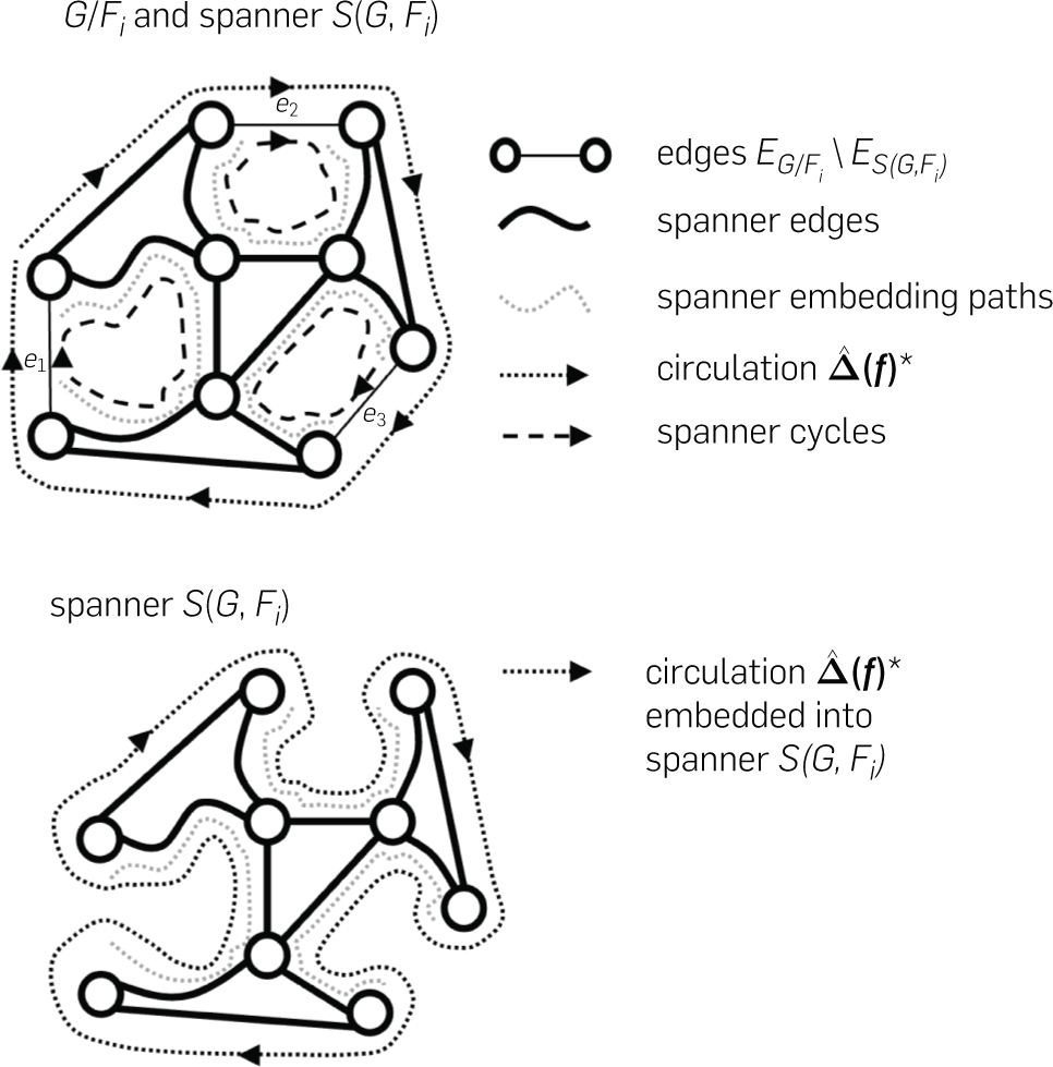
We maintain a recursive hierarchy of graphs. At the top level of our hierarchy, for the input graph G, we produce B = O(log n) core graphs. To obtain each such core graph, for each i∈[B], we sample a (random) forest Fi with Õ(m/k) connected components for some size reduction parameter k. The associated core graph is the graph G/Fi which denotes G after contracting the vertices in the same components of Fi. We can define a map that lifts circulations in the core graph G/Fi, to circulations Δ in the graph G by routing flow along the contracted paths in Fi. The lengths in the core graph (again let ) are chosen to upper bound the length of circulations when mapped back into G such that . Crucially, we must ensure these new lengths do not stretch the witness circulation Δ⋆ when mapped into G/Fi by too much, so we can recover it from G/Fi. To achieve this goal, we choose Fi to be a low-stretch forest, that is, a forest with properties similar to those of a low-stretch tree. In Section 2.3, we summarize the central aspects of our core graph construction.
While each core graph G/Fi now has only Õ(m/k) vertices, it still has m edges which are too large for our recursion. To overcome this issue we build a spanner on S(G, Fi) on G/Fi to reduce the number of edges to Õ(m/k), which guarantees that for every edge e = (u, v) that we remove from G/Fi to obtain S(G, Fi), there is a u-to-v path in S(G, Fi) of length mo(1). Ideally, we would now recurse on each spanner S(G, Fi), again approximating it with a collection of smaller core graphs and spanners. However, we face an obstacle: removing edges could destroy the witness circulation so that possibly no good circulation exists in any S(G, Fi). To solve this problem, we compute an explicit embedding that maps each edge e=(u, v)∈G/Fi to a short u-to-v path in S(G, Fi). We can then show the following dichotomy: Let denote the witness circulation when mapped into the core graph G/Fi. Then, either one of the edges has a spanner cycle consisting of e combined with which is almost as good as , or re-routing into S(G, Fi) roughly preserves its quality. Figure 3 illustrates this dichotomy. Thus, either we find a good cycle using the spanner, or we can recursively find a solution S(G, Fi) onthat almost matches in quality. To construct our dynamic spanner with its efficient updates and strong stability guarantees under changes in the input graph, we design a new approach that diverges from other recent works on dynamic spanners.
Our recursion uses d levels, where we choose the size reduction factor k such that kd ≈ m and the bottom level graphs have mo(1) edges. Note that since we build B trees on G and recurse on the spanners of G/F1, G/F2, …, G/FB, our recursive hierarchy has a branching factor of B = O(log n) at each level of recursion. Thus, choosing , we get Bd = mo(1) leaf nodes in our recursive hierarchy. Now, consider the forests on the path from the top of our recursive hierarchy to a leaf node. We can patch these forests together to form a tree associated with the leaf node. For each of these trees, we maintain a link-cut tree data structure. Using this data structure, whenever we find a good cycle, we can route flow along it and detect edges where the flow has changed significantly. The cycles are either given by an off-tree edge or a collection of mo(1) off-tree edges coming from a spanner cycle. We call the entire construction a branching tree chain. In Section 2.4, we elaborate on the overall composition of the data structure.
What have we achieved using this hierarchical construction compared to our simple, static algorithm? First, consider the setting of an oblivious adversary, where the gradient and length update sequences and the optimal circulation after each update are fixed in advance (i.e., the adversary is oblivious of the algorithm’s random choices). In this setting, we can show that our spanner-of-core graph construction can survive through m1−o(1)/ki updates at level i. Meanwhile, we can rebuild these constructions in time m1+o(1)/ki−1, leading to an amortized cost per update of kmo(1) ≤ mo(1) at each level. This gives the first dynamic data structure for our undirected min-ratio problem with mo(1) query time against an oblivious adversary.
However, our real problem is harder: the witness circulation in each round is Δ(f)⋆ = f⋆ − f and depends on the updates we make to f, making our sequence of subproblems adaptive. While we cannot show that our data structure succeeds against an adaptive adversary, we give a data structure that works against a restricted adaptive adversary. We show that the witness circulation f⋆ − f lets us express the IPM as such a restricted adversary.
2.3. Building core graphs
In this section, we describe our core graph construction, which maps our dynamic undirected min-ratio cycle problem on a graph G with at most m edges and vertices into a problem of the same type on a graph with only Õ(m/k) vertices and m edges, and handles Õ(m/k) updates to the edges before we need to rebuild it.
Forest routings and stretches.
To understand how to define the stretch of an edge e with respect to a forest F, it is useful to define how to route an edge e in F. Given a spanning forest F, every path and cycle in G can be mapped to G/F naturally (where we allow G/F to contain self-loops). On the other hand, if every connected component in F is rooted, where denotes the root corresponding to a vertex u ∈ V, we can map every path and cycle in G/F back to G as follows. Let P = e1, …, ek be any (not necessarily simple) path in G/F where the preimage of every edge ei is . The preimage of P, denoted PG, is defined as the following concatenation of paths:
where we use A ⊕ B to denote the concatenation of paths A and B, and F[a, b] to denote the unique ab-path in the forest F. When P is a circuit (i.e., a not necessarily simple cycle), PG is a circuit in G as well. One can extend these maps linearly to all flow vectors and denote the resulting operators as ΠF: ℝE(G) → ℝE(G/F) and . Since we let G/F have self-loops, there is a bijection between the edges of G and G/F, and thus ΠF acts like the identity function. Related routing schemes date back to Spielman-Teng34 and are generally known as portal routing.
To make our core graph construction dynamic, the key operation we need to support is the dynamic addition of more root nodes, which results in forest edges being deleted to maintain the invariant each connected component has a root node. Whenever an edge is changing in G, we ensure that G/F approximates the changed edge well by forcing both its endpoints to become root nodes, which in turn makes the portal routing of the new edge trivial and this guarantees its stretch is 1.
For any edge eG = (uG, vG) in G with image e in G/F, we set , the edge length of e in G/F, to be an upper bound on the length of the forest routing of e, that is, the path . Meanwhile, we define , as an overestimate on the stretch of e w.r.t. the forest routing. A priori, it is unclear how to provide a single upper bound on the stretch of every edge, as the root nodes of the endpoints are changing over time. Providing such a bound for every edge is important for us as the lengths in G/F could otherwise be changing too often when the forest changes. We guarantee these bounds by a scheme that makes auxiliary edge deletions in the forest in response to external updates, with the resulting additional roots chosen carefully to ensure the length of upper bounds.
Now, for any flow f in G/F, its length in G/F is at least the length of its pre-image in G, that is, . Let Δ⋆ be the optimal solution to Equation (2). We will show later how to build F such that with constant probability holds for some γ = mo(1), solving Equation (2) on G/F with edge length and properly defined gradient ĝ on G/F yields an -approximate solution for G. The gradient ĝ is defined so that the total gradient of any circulation Δ on G/F and its preimage in G is the same, that is, . The idea of incorporating gradients into portal routing was introduced in Kyng et al.24; our version of this construction is somewhat different to allow us to make it dynamic efficiently.
Collections of low stretch decompositions (LSD).
The first component of the data structure is constructing and maintaining forests of F that form a Low Stretch Decomposition (LSD) of G. Informally, a k-LSD is a rooted forest F ⊆ G that decomposes G into O(m/k) vertex disjoint components. Given some positive edge weights and reduction factor k > 0, we compute a k-LSD F and length upper bounds of G/F that satisfy two properties:
for any edge eG ∈ G with image e in G/F, and
The weighted average of w.r.t. v is only Õ(1) that is, .
Item 1 guarantees that the solution to Equation (2) for G/F yields a Õ(k)-approximate one for G. However, this guarantee is not sufficient for our data structure, as our B-branching tree chain has d ≈ logk m levels of recursion and the quality of the solution from the deepest level would only be Õ(k)d≈m1+o(1)-approximate.
Instead, we compute k different edge weight assignments v1, …, vk via multiplicative weight updates so that the LSDs F1, …, Fk have Õ(1) an average stretch on every edge in , for all eG ∈ G with image e in G/F.
By Markov’s inequality, for any fixed flow f in holds for at least half the LSDs corresponding to F1, …, Fk. Taking O(log n) samples uniformly from F1, …, Fk, say F1, …, FB for B = O(log n) we get that with high probability
(3)That is, it suffices to solve Equation (2) on G/F1, …, G/FB to find an Õ(1)-approximate solution for G.
2.4. Maintaining a branching tree chain
Our branching chain is constructed as follows:
Sample and maintain B = O(log n) k-LSDs F1, F2, …, FB, and their associated core graphs G/Fi. Across O(m/k) updates at the top level, the forests Fi are decremental, that is, only undergo edge deletions (from root insertions), and will have Õ(m/k) connected components.
Maintain spanners S(G, Fi) of the core graphs G/Fi, and embeddings , say with length increase γℓ = mo(1).
Recursively process the graphs S(G, Fi), that is, maintain LSDs and core graphs on those, and spanners on the contracted graphs, etc., for d total levels, with kd = m.
Whenever a level i accumulates m/ki total updates, hence doubling the number of edges in the graphs at that level, we rebuild levels i, i + 1, …, d.
Recall that on average, the LSDs stretch lengths by Õ(1), and the spanners S(G, Fi) stretch lengths by γℓ. Hence, the overall data structure stretches lengths by Õ(γℓ)d = mo(1) (for appropriately chosen d).
We now discuss how to update the forests G/Fi and spanners S(G, Fi). Intuitively, every time an edge e = (u, v) is changed in G, we will delete Õ(1) additional edges from Fi. This ensures that no edge’s total stretch/routing-length increases significantly due to the deletion of e. As the forest Fi undergoes edge deletions, the graph G/Fi undergoes vertex splits, where a vertex has a subset of its edges moved to a newly created vertex. Thus, a key component of our data structure is to maintain spanners and embed-dings of graphs undergoing vertex splits (and edge insertions/ deletions). Importantly, the amortized recourse (number of changes) to the spanner S(G, Fi) is mo(1) independent of k, even though the average degree of G/Fi is Ω(k). Hence, on average Ω(k) edges will move in G/Fi per vertex split.
Overall, let every level have recourse γr = mo(1) (independent of k) per tree. Then each update at the top level induces O(Bγr)d (as we branch using B forests/core graphs at each level of the recursion) updates in the data structure overall. Intuitively, for the proper choice of d = ω(1), both the total recourse O(Bγr)d and approximation factor Õ(γℓ)d are mo(1) as desired.
2.5. Going beyond oblivious adversaries by using IPM guarantees
The precise data structure in the previous section only works for oblivious adversaries, because we used that if we sampled B = O(log n) LSDs, then w.h.p. there is a tree whose average stretch is Õ(1) with respect to a fixed flow f. However, since we are updating the flow along the circulations returned by our data structure, we influence future updates, so the optimal circulations our data structure needs to preserve, are not independent of the randomness used to generate the LSDs. To overcome this issue, we leverage the key fact that the flow f⋆ − f is a good witness for the min-ratio cycle problem at each iteration.
To simplify our discussion, we focus on the role of the witness in ensuring the functioning of a single layer of core graph construction, which already captures the main ideas. We can prove that for any flow f, g(f)⊤ Δ(f)/(100m+∥L(f)Δ(f)∥1) ≤ −Ω̃(1) holds where Δ(f) = f⋆ − f. Then, the best solution to Equation (2) among the LSDs G/F1, …, G/FB maintains an Õ(1)-approximation of the quality of the witness Δ(f) = f⋆ − f as long as
(4)In this case, let be the best solution obtained from graphs G/F1, …, G/FB. We have
The additive term is there for technical reasons that can be ignored for now. We define the width w(f) of Δ(f) as w(f) = 100 · 1+|L(f)Δ(f)|. The name comes from the fact that w(f)e is always at least for any edge e. We show that the width is also slowly changing across IPM iterations, in that if the width changed by a lot, then the residual capacity of e must have changed significantly. This gives our data structure a way to predict which edges’ contribution to the length of the witness flow f⋆ − f could have significantly increased.
Observe that for any forest Fj in the LSD of G, we have . Thus, we can strengthen Equation (4) and show that the IPM potential can be decreased by m−o(1) if
Equation (5) also holds with w.h.p. if the collection of LSDs is built after knowing f. However, this does not necessarily hold after augmenting with Δ, an approximate solution to Equation (2).
Due to the stability of w(f), we have w(f + Δ)e ≈ w(f)e for every edge e whose length does not change a lot. For other edges, we update their edge length and force the stretch to be 1, that is, via the dynamic LSD maintenance, by shortcutting the routing of the edge e at its endpoints. To distinguish between the earlier stretch values and those after updating edges, let us denote the former by and the latter by . This gives that for any j∈[B], the following holds:
Using the fact that , we have the following:
Thus, solving Equation (2) on the updated G/F1, …, G/FB yields a good enough solution for reducing IPM potential as long as the width of w(f + Δ) has not decreased significantly, that is, ∥w(f)∥1 ≤ Õ(1)∥w(f + Δ)∥1.
If the solution on the updated graphs G/F1, …, G/FB does not have a good enough quality, we know by the above discussion that ∥w(f + Δ)∥1 ≤ 0.5∥w(f)∥1 must hold. Then, we re-compute the collection of LSDs of G and solve Equation (2) on the new collection of G/F1, …, G/FB again. Because each recomputation reduces the ℓ1 norm of the width by a constant factor, and all the widths are bounded by exp(logO(1) m) (which can be guaranteed by the IPM), there can be at most Õ(1) such recomputations. At the top level, this only increases our runtime by Õ(1) factors.
The full construction is along these lines, but more complicated since we recursively maintain the solutions on the spanners of each core graph G/F1, …, G/FB. In the full version of the paper, we describe and analyze a multi-level rebuilding scheme that extends the above reasoning to our full data structure.
3. Conclusion
In this paper, we presented an almost-linear time algorithm for minimum-cost flow, maximum flow, and more generally, all convex single-commodity flows. Our work essentially settles the complexity of several fundamental and intensely studied problems in algorithms design. We hope that the ideas introduced in this work will spur further research in several directions, including simpler and faster algorithms for flow problems; hopefully resulting in a significant impact on algorithms in practice.
Acknowledgments
Li Chen was supported by NSF Grant CCF-2106444. Rasmus Kyng and Maximilian Probst Gutenberg have received funding from the grant “Algorithms and complexity for high-accuracy flows and convex optimization” (no. 200021 204787) of the Swiss National Science Foundation. Yang P. Liu was supported by NSF CAREER Award CCF-1844855 and NSF Grant CCF-1955039. Richard Peng was partially supported by NSF CAREER Award CCF-1846218 and NSERC Discovery Grant RGPIN-2022–03207. Sushant Sachdeva’s research is supported by a Natural Sciences and Engineering Research Council of Canada (NSERC) Discovery Grant RGPIN-2018–06398 and an Ontario Early Researcher Award (ERA) ER21–16–284.
The authors thank the 2021 Hausdorff Research Institute for Mathematics Program Discrete Optimization. The authors are very grateful to Yin Tat Lee and Aaron Sidford for several useful discussions.


Join the Discussion (0)
Become a Member or Sign In to Post a Comment