Abstract
Numerous microarchitectural optimizations unlocked tremendous processing power for deep neural networks that in turn fueled the AI revolution. With the exhaustion of such optimizations, the growth of modern AI is now gated by the performance of training systems, especially their data movement. Instead of focusing on single accelerators, we investigate data-movement characteristics of large-scale training at full system scale. Based on our workload analysis, we design HammingMesh, a novel network topology that provides high bandwidth at low cost with high job scheduling flexibility. Specifically, HammingMesh can support full bandwidth and isolation to deep learning training jobs with two dimensions of parallelism. Furthermore, it also supports high global bandwidth for generic traffic. Thus, HammingMesh will power future large-scale deep learning systems with extreme bandwidth requirements.
1 Motivation
Artificial intelligence (AI) is experiencing unprecedented growth providing seemingly open-ended opportunity. Deep learning models combine many layers of operators into a complex function that is trained by optimizing its parameters to large datasets. Given the abundance of sensor, simulation, and human artifact data, this new model of designing computer programs, also known as data-driven programming or “software 2.0”, is mainly limited by the capability of machines to perform the compute- and data-intensive training jobs. In fact, the predictive quality of models improves as their size and training data grow to unprecedented scales.15 Building deep learning supercomputers, to both explore the limits of artificial intelligence and commoditize it, is becoming not only interesting to big industry but also humanity as a whole.
A plethora of different model types exist in deep learning and new major models are developed every two to three years. Yet, their computational structure is similar—they consist of layers of operators and they are fundamentally data-intensive.14 Many domain-specific accelerators take advantage of peculiarities of deep learning workloads be it matrix multiply units (“tensor cores”), specialized vector cores, or specific low-precision datatypes. Those optimizations can lead to orders of magnitude efficiency improvements. Yet, as we are approaching the limits of such microarchitectural improvements, we need to direct our focus to the system level.
Today’s training jobs are already limited by data movement.14 In addition, trends in deep neural networks, such as sparsity, further increase those bandwidth demands in the near future.9 Memory and network bandwidth are expensive—in fact, they form the largest cost component in today’s systems. Standard HPC systems with the newest InfiniBand adapters can offer 400Gb/s but modern deep learning training systems offer much higher bandwidths. Google’s TPUv2, designed seven years ago, has 1Tbps off-chip bandwidth, AWS’ Trainium has up to 1.6Tbps per Tm1n instance, and Nvidia A100 and H100 chips have 4.8 and 7.2Tbps (local) NVLINK connectivity, respectively. The chips in Tesla’s Dojo deep learning supercomputer even have 128Tbps off-chip bandwidth—more than a network switch. Connecting these extreme-bandwidth chips at reasonable cost is a daunting task and today’s solutions, such as NVLINK, provide only local islands of high bandwidth.
We argue that general-purpose HPC and datacenter topologies are not cost-effective at these endpoint injection bandwidths. Yet, workload specialization, similar to existing microarchitectural optimizations, can lead to an efficient design that provides the needed high-bandwidth networking. We begin with developing a generic model that accurately represents the fundamental data movement characteristics of deep learning workloads. Our model shows the inadequacy of the simplistic view that the main communication in deep learning is allreduce. In fact, we show that communication can be expressed as a concurrent mixture of pipelines and orthogonal reductions forming toroidal data movement patterns. This formulation shows that today’s HPC networks, optimized for full global (bisection) bandwidth, are inefficient for deep learning workloads. Specifically, their global bandwidth is overprovisioned while their local bandwidth is underprovisioned.
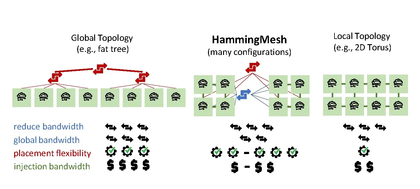
We use our insights to develop HammingMesh, a flexible topology that can adjust the ratio of local and global bandwidth for deep learning workloads. HammingMesh combines ideas from torus and global-bandwidth topologies (for example, fat tree) to enable a flexibility-cost tradeoff shown schematically in Figure 1. Inspired by machine learning traffic patterns, HammingMesh connects local high-bandwidth 2D meshes using row and column (blue and red) switches into global networks.a
In summary, we show how deep learning communication can be modeled as sets of orthogonal and parallel Hamiltonian cycles to simplify mapping and reasoning. Based on this observation, we define principles for network design for deep learning workloads. Specifically, our HammingMesh topology
uses technology-optimized local (for example, PCB board) and global (optical, switched) connectivity.
utilizes limited packet forwarding capabilities in the network endpoints to achieve lower cost and higher flexibility.
enables full-bandwidth embedding of virtual topologies with deep learning traffic characteristics.
supports flexible job allocation even with failed nodes.
enables flexible configuration of oversubscription factors to adjust global bandwidth.
With those principles, HammingMesh enables extreme off-chip bandwidths to nearest neighbors at more than 8x cheaper allreduce bandwidth compared to standard HPC topologies such as fat trees. HammingMesh reduces the number of external switches and cables and thus reduces overall system cost. Furthermore, it provides significantly higher flexibility than torus networks. HammingMesh also enables seamless scaling to larger domains without separation between on- and off-chassis programming models (like NVLINK vs. InfiniBand). And last but not least, we believe that HammingMesh topologies extend to other machine learning, (multi)linear algebra, parallel solvers, and many other workloads with similar traffic characteristics.
We start with a characterization of parallel deep learning and the related data movement patterns. For reference, we provide an overview of symbols used in this paper in Table 1.
| Symbol | Description |
|---|---|
| M | number of examples per minibatch |
| NP | number of network parameters |
| W | size of a word |
| D, P, O | degree of data, pipeline, operator parallelism |
| a, b and x, y | 2D HammingMesh board and global sizes |
2 Communication in Distributed Deep Learning
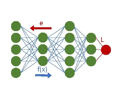
One iteration of deep learning training with Stochastic Gradient Descent (SGD) consists of two phases: the forward pass and the backward pass. The forward pass evaluates the network function f(x) on a set of M examples, also called a “minibatch”. The backward pass of SGD computes the average loss L and propagates the errors e backwards through the network to adapt the parameters P. This training process proceeds through multiple (computationally identical) iterations until the model achieves the desired accuracy.
Parallelism and data distribution can fundamentally be arranged along three axes: data parallelism, pipeline parallelism, and operator parallelism.5 The latter two are often summarized as model parallelism and operator parallelism is sometimes called tensor parallelism. We now briefly discuss their main characteristics.
2.1 Data parallelism.
When parallelizing over the training data, we train D separate copies of the model, each with different examples. To achieve exactly the same result as in serial training, we sum the distributed gradients before applying them to the weights at the end of each iteration. If the network has NP parameters, then the communication volume of this step is WNP.
Modern deep neural networks have millions or billions of parameters, making this communication step expensive. Thus, many optimizations target gradient summation22—some even change convergence properties during the training process but maintain final result quality.2 Dozens of different techniques have been developed to optimize this communication—however, all perform some form of distributed summation operation like MPI_Allreduce. Data-parallelism differs thus mostly in the details such as invocation frequency, consistency, and sparsity.
2.2 Pipeline parallelism.
Deep neural networks are evaluated layer by layer with the outputs of layer i feeding as inputs into layer i + 1. Back-propagation is performed along the reverse direction starting at the loss function L after the last layer and proceeding from layer i + 1 to layer i. We can model the network as a pipeline with P stages with one or more layers per stage. Forward and backward passes can be interleaved at each processing element to form a bidirectional training pipeline. Pipelines suffer from characteristic start-up and tear-down overheads. These can be reduced by running two pipelines in both directions19 or by using asynchronous schemes that impact convergence.
Overall, pipelining schemes can use P processors with a nearest-neighbor communication volume proportional to the number of output activations at the cut layers.
2.3 Operator parallelism.
Very large layer computations (operators) can be distributed to O processors. Most deep learning layer operators follow computational schedules of (multi-)linear algebra and tensor contractions and require either (tightly coupled) distributed reductions or nearest-neighbor communications.
2.4 Overall communication pattern.
When all forms of parallelism are used, then the resulting job comprises D × P × O accelerators; each accelerator in a job has a logical address (1..D, 1..P, 1..O). The data-, pipeline-, and operator-parallel communication can be arranged as one-dimensional slices (rings) by varying only one coordinate of the Cartesian structure. Pipelines would leave one connection of the ring unused. For example, the data-parallel dimension consists of P · O rings of length D each. Each of those rings represents a single allreduce. We show efficient ring-based reduction and broadcast algorithms for large data volumes in Section 4.1.2.
The overall composition of communication patterns forms a torus as illustrated in the right part of Figure 2 for a 3×3×3 example: Both the operator and the data parallel dimensions use nine simultaneous allreductions of size three each. The pipeline parallel dimension uses nine three-deep pipelines on three different model replicas, each split in three pieces.
While we can map such a logical torus to a full-bandwidth network topology, it seems wasteful to provide full bandwidth for sparse communication. For example, a 400Gb/s non-blocking fat tree with 16,384 endpoints provides full bisection bandwidth of more than . A bi-directional 32x32x16 torus communication pattern requires at most 32 · 16 · 2 · 50GB/s= 51.2TB/s bisections (cutting one dimension of size 32)—a mere 12.5% of the offered bandwidth. In other words, 88% of the available bandwidth will remain unused and is wasted. Furthermore, it is not always simple to map such torus communication patterns efficiently to full-bandwidth low-diameter topologies in practice.
3 HammingMesh
Based on the communication workload analysis, we now design a flexible and efficient network topology. The basic requirements are to support highest injection bandwidth for a set of jobs, each following a virtual toroidal communication topology. We note that medium-size models are often decomposed only in two dimensions in practice (usually data and pipeline or data and operator). Only extreme-scale workloads require all three dimensions—even then, communication along the data parallel dimension only happens after one complete iteration. Thus, we use a two-dimensional physical topology.
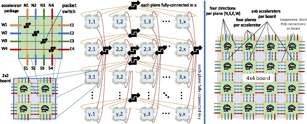
As a case study, we assume a modern deep learning accelerator package with 16 400Gb/s off-chip network links, a total network injection bandwidth of 800GB/s (top left in Figure 3). Our topology design also takes technology costs into account: Similar to Dragonfly, which combines local short copper cables with global long fiber cables to design a cost-effective overall topology, we combine such local groups with a global topology. Different from Dragonfly, we choose two quite distinct topologies: The local groups are formed by a local inexpensive high-bandwidth 2D mesh using short metal traces on PCB boards. This is the opposite of Dragonfly designs, which combine densely-connected local groups (“virtual switches”) and connect those fully globally. HammingMesh combines sparsely connected boards in a dimension-wise (not globally) fully-connected topology. Those boards are connected by a two-dimensional Hamming graph, in which each dimension is logically fully connected (for example, by a fat tree). All accelerator ports are arranged in planes with four directions each. Our example accelerator has four planes (top left in Figure 3), for example, plane 1 has ports E1, W1, N1, and S1. We assume that each accelerator can forward packets within a plane like any network switch. Accelerators do not have to forward packets between planes, for example, packets arriving at N1 may only be forwarded to E1, W1, or S1 but none of the other ports. Thus, only simple 4×4 switches are needed at each accelerator. Figure 3 illustrates the structure in detail.
A 2D HammingMesh is parameterized by its number of planes and four additional numbers: (a, b), the dimensions of the board, and (x, y), the dimensions of the global topology. It connects a total of abxy accelerators. We abbreviate HammingMesh with HxMesh in the following. Furthermore, an HxMesh with an a × b accelerator board is called HaxbMesh, for example, for a 2×2 board, H2x2Mesh. For square board topologies, we skip the first number, for example, an H2x2Mesh that connects 10×10 boards is called a 10×10 Hx2Mesh.
HxMesh has a large design space: We can combine different board and global topologies, for example, 3D mesh boards with global Slim Fly topologies.6 In this work, we consider 2D boards as most practical for PCB traces. The board arrangement could be reduced to a 1D HxMesh, where y = 1 and each Nk link is connected to the corresponding Sk link (“wrapped around”). The same global topology can also span multiple rows or columns (for example, full boards in a single fat tree). For ease of exposition, we limit ourselves to 2D HxMeshes using 2D boards and row/column-separated global topologies. We use two-level fat trees as global topologies to connect the boards column and row wise. If the boards can be connected with a single 64-port switch, we use that instead of a fat tree.
3.1 Bisection and global bandwidth.
Bisection cut is defined as the minimal number of connections that would need to be cut in order to bisect the network into two pieces, each with an equal number of accelerators. The bisection bandwidth is the cut multiplied by the link bandwidth. Let us assume a single-plane of an x × y HxaMesh (square board) with x ≤ y and y even, wlog. We now consider the xy/2 “lower” half boards with y coordinates 1, 2, … y/2. We split the HxMesh into two equal pieces by cutting the 2a links in y direction of each of the lower half of the boards. This results in a total cut width of axy. Each accelerator has four network links per plane, a total injection bandwidth of 4a2 per board. We have xy/2 boards with a total injection bandwidth of 4a2xy/2 = 2xya2 in each partition. Thus, the relative bisection bandwidth is axy/2xya2 = 1/2a.
In a bisection traffic pattern, all traffic crosses the network bisection (any two communicating endpoints are in different sets of the bisection). Such (worst-case) patterns are rare in practice. A more useful pattern, more often observed in practice is alltoall, where each process sends to all other processes. This pattern is the basis of parallel transpositions, Fast Fourier Transforms, and many graph algorithms. The achievable theoretical bandwidth for such alltoall patterns is often called “global bandwidth”. Some topology constructions take advantage of the fact that global bandwidth is higher than bisection bandwidth. Prisacari et al.21 shows that full-global bandwidth (alltoall) fat trees can be constructed with 25% less switches than nonblocking fat trees. Dragonfly,17 Slim Fly,6 or other low-diameter topologies16 can further reduce the number of switches in very large installations while maintaining full global bandwidth. As is customary for low-diameter topologies,6,17 we assess it using packet-level simulations of alltoall traffic.
3.2 Example topologies.
We consider a small cluster with approximately 1,000 accelerators and a large cluster with approximately 16,000 accelerators as specific design points to compare realistic networks. We compare various fat trees (nonblocking, 50%, 75% tapered), full bandwidth Dragonfly, two-dimensional torus, and HyperX,b with Hx2Mesh and Hx4Mesh example topologies.
Table 2 summarizes the main cost and bandwidth results. Global and allreduce bandwidth are determined using packet-level simulations (see Section 4) for large messages. For all experiments, we simulated a single plane of HammingMesh and four planes for all other topologies, i.e., a total injection bandwidth of 4×400Gb/s. We use industry-standard layouts and cable configurations for the cost estimates: fat trees are tapered beginning from the second level and connect all endpoints using DAC and all switches using AoC. Dragonfly topologies use full-bandwidth groups with a = 16 routers each, p = 8 endpoints per router, and h = 8 links to other groups with DAC links inside the groups and AoC links between groups. The torus uses 2 × 2 board topologies with discounted local PCB connectivity, similar to Hx2Mesh and only DAC cables between the boards. For HxMeshes, we use DAC links to connect endpoints to switches along one dimension, and AoC links for the other dimension. All inter-switch links are AoC as in fat trees.
| Topology | Small Cluster (≈1,000 accelerators) | Large Cluster (≈16,000 accelerators) | ||||||||||
|---|---|---|---|---|---|---|---|---|---|---|---|---|
| cost | glob. BW | global | ared. BW | ared. | diam. | cost | glob. BW | global | ared. BW | ared. | diam. | |
| [M$] | [% inject] | saving | [% peak] | saving | [M$] | [% inject] | saving | [% peak] | saving | |||
| nonbl. FT | 25.3 | 99.9 | 1.0x | 98.9 | 1.0x | 4 | 680 | 98.9 | 1.0x | 99.8 | 1.0x | 6 |
| 50% tap. FT | 17.6 | 51.2 | 0.7x | 98.9 | 1.4x | 4 | 419 | 47.6 | 0.8x | 99.8 | 1.6x | 6 |
| 75% tap. FT | 13.2 | 25.7 | 0.5x | 98.9 | 1.9x | 4 | 271 | 24 | 0.6x | 99.8 | 2.5x | 6 |
| Dragonfly | 27.9 | 62.9 | 0.6x | 98.8 | 0.9x | 3 | 429 | 71.5 | 1.2x | 98.6 | 1.6x | 5 |
| 2D HyperX | 10.8 | 91.6 | 2.1x | 98.1 | 2.3x | 4 | 448 | 95.8 | 1.5x | 99.2 | 1.5x | 8 |
| Hx2Mesh | 5.4 | 25.4 | 1.2x | 98.3 | 4.7x | 4 | 224 | 25 | 0.8x | 92.3 | 2.8x | 8 |
| Hx4Mesh | 2.7 | 11.3 | 1.0x | 98.4 | 9.3x | 8 | 43.3 | 10.5 | 1.7x | 98 | 15.4x | 8 |
| 2D torus | 2.5 | 2 | 0.2x | 98.1 | 10.1x | 32 | 39.5 | 1.1 | 0.2x | 99.2 | 17.1x | 128 |
3.3 Logical job topologies and failures in HxMesh.
As we discussed in Section 2.4, communication patterns in deep learning can be modeled as sets of cycles. Typical learning jobs use either logical 1D cycles for small models with only data parallelism or 2D tori that combine data and pipeline parallelism for medium-scale models or combining pipeline and model parallelism for very large models. Each specific training job will have a different optimal decomposition resulting in 1D, 2D, or sometimes even 3D logical communication topologies.
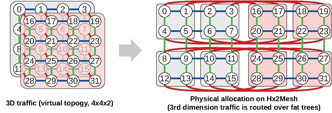
We use logical 2D topologies for our training jobs. Each job uses several boards and requests a u × v layout (that is, a, b divides u, v, respectively). If the application topology follows a 1D or 3D scheme, then users use standard folding techniques to embed it into two dimensional jobs. Figure 4 shows an example of 3D virtual topology mapped on an Hx2Mesh physical topology. Processes can be sliced on the third dimension and mapped on different boards. Communications between different slices of the third dimension are routed over the per-column or per-row fat trees, depending how different slices are mapped. To minimize communication latency between slices, consecutive slices should be adjacent to each other.
It is easy to see that any consecutive u × v block of boards in a 2D HxMesh has the same properties as a full u × v HxMesh. We call such subnetworks virtual sub-HxMeshes. They are a major strength of HxMesh compared to torus networks in terms of fault tolerance as well as for allocating jobs. In fact, HxMeshes major strength compared to torus networks is that virtual subnetworks can be formed with non-consecutive sets of boards (not only blocks): any set of boards in an HxMesh where all boards that are in the same row have the same sequence of column coordinates can form a virtual subnetwork. We will show examples below together with a motivation for subnetworks—faults.
Fault-tolerance. We assume that a board is the unit of failure in an HxMesh, that is, if an accelerator or link in a board fail, the whole board is considered failed. This simplifies system design and service. Partial failure modes (for example, per plane) are outside the scope of this work.
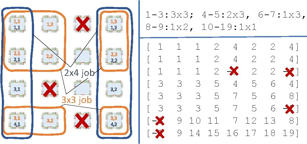
The left part of Figure 5 shows a 4×4 Hx2Mesh and three board failures. We show two different subnetworks (many more are possible): a 2×4 subnetwork (blue) with the physical boards (1, 1), (1, 4), (2, 1), (2, 4), (3, 1), (3, 4), (4, 1), (4, 4) and a 3×3 subnetwork (yellow) with the physical boards (1, 1), (1, 2), (1, 4), (2, 1), (2, 2), (2, 4), (4, 1), (4, 2), (4, 4). We also annotate the new coordinates of boards in the virtual subnetworks. Remapping can be performed transparently to the user application, which does not observe a difference between a virtual and physical HxMesh in terms of network performance. The right part of the figure shows the output of our automatic mapping tool (described in detail in the full version of this paper10) for a more complex configuration of jobs (top, read job ids 1-3 are 3 × 3 logical jobs, and so on).
4 Results and Comparison
We now evaluate HxMesh topology options in comparison with all topologies listed in Table 2. We use the Structural Simulation Toolkit (SST),1 a packet-level network simulator, which has been validated against the Cray Slingshot interconnect.8 SST enables us to reproduce the behavior of full MPI applications directly in the simulation environment where they react to dynamic network changes (for example, congestion). In total, we ran simulations of more than 120 billion packets using more than 0.6 million core hours with parallel simulations. We select various representative microbenchmarks and scenarios for deep learning jobs and publish the full simulation infrastructure such that readers can simulate their own job setup.
4.1 Microbenchmarks.
We start by analyzing well-known microbenchmark traffic patterns to assess and compare achievable peak bandwidth.
4.1.1 Global traffic patterns.
We first investigate global traffic patterns such as alltoall and random permutations as global-traffic workloads. We note that HammingMesh is not optimized for those patterns as they are rare on deep learning traffic.
Alltoall. Alltoall sends messages from each process to all other processes. In our implementation, each of the p processes performs p − 1 iterations. In each iteration i, process j sends to process j + i mod p in a balanced shift pattern.
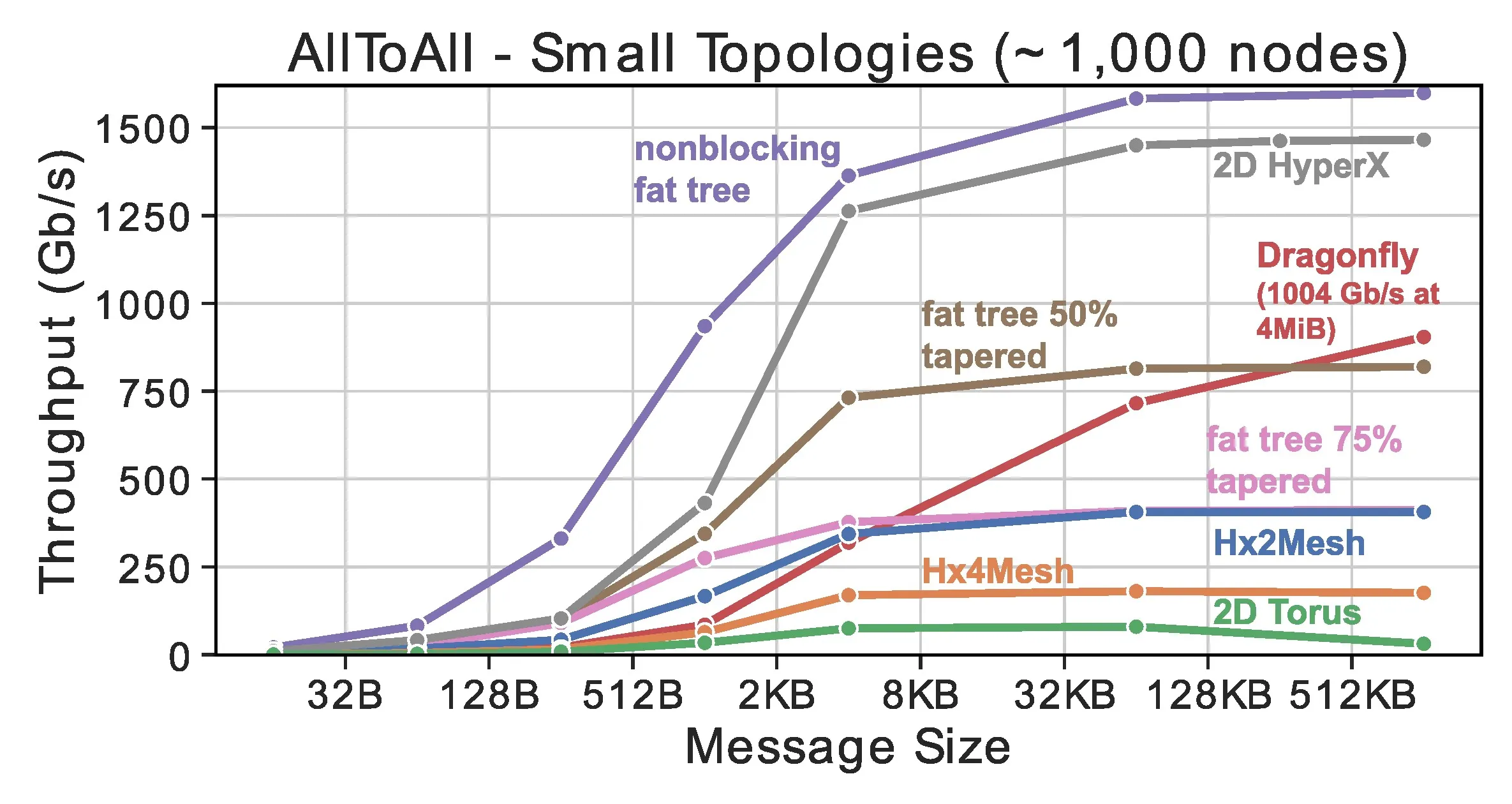
Table 2 shows the results for 1 MiB messages while Figure 6 shows the global bandwidth at different message sizes. Small Hx2 and Hx4Meshes achieve bandwidths around the cut width of 1/4 and 1/8, respectively (cf. Section 3.1). This is because not all global traffic crosses the bisection cuts, especially for smaller clusters. The large cluster configuration performs closer to those bounds and loses some bandwidth due to adaptive routing overheads. Despite its lower bandwidth, even large HxMeshes remain competitive in terms of cost-per global bandwidth and some are even more cost effective on global bandwidth than fat trees.
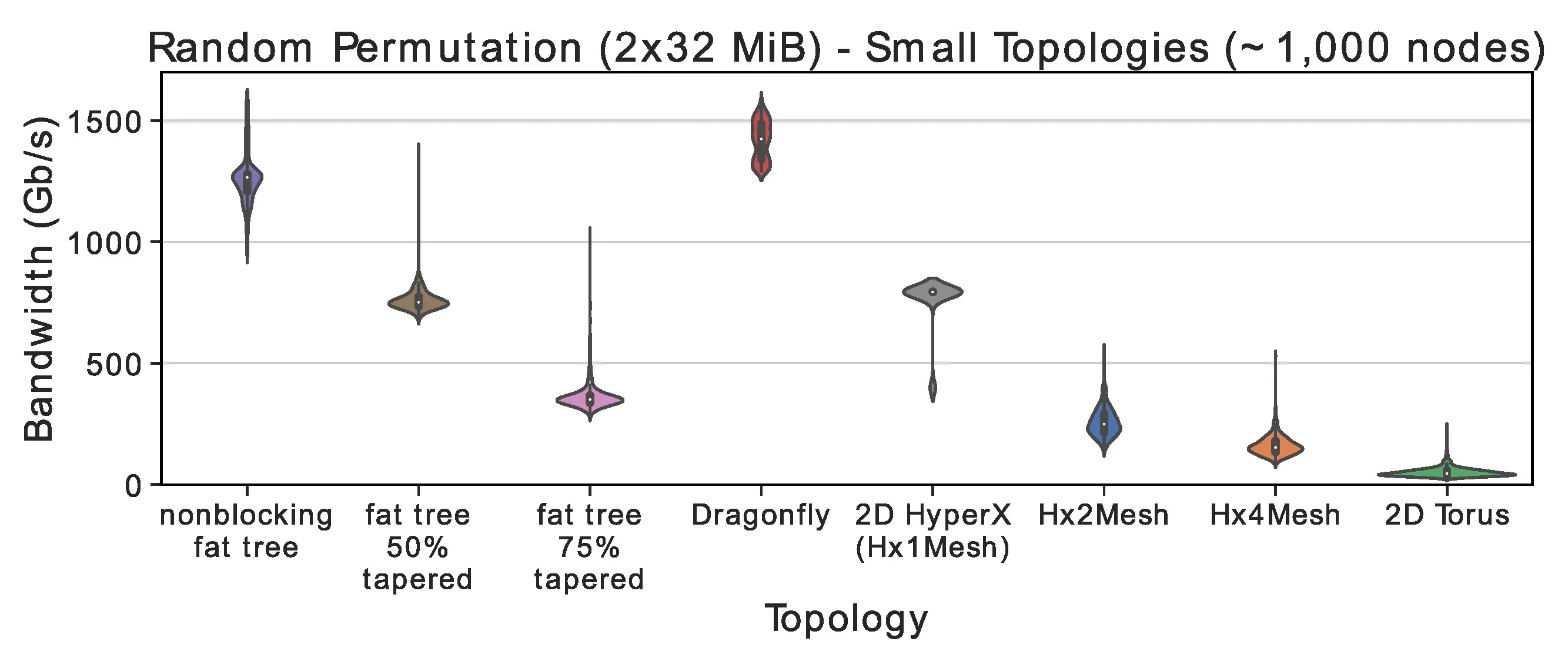
Random permutation. In permutation traffic, each accelerator selects a unique random peer to send to and receive from. Here, the achieved bandwidth also depends on the location of both peers. Figure 7 shows the distributions of receive bandwidths across all of the 1k accelerators in the small cluster configurations.
Our results indicate that all topologies have significant variance across different connections (between different node pairs), which makes job placement and locality significant. HxMeshes are among the most cost effective topologies.
4.1.2 Reduction traffic patterns.
We distinguish three fundamental algorithm types: trees, pipelines, and near-optimal full-global bandwidth algorithms.
Simple trees. For small data, simple binary or binomial tree reductions are the best choice. They perform a reduction of S bytes on p processors in time T ≈ log2 (p)α + log2 (p)Sβ.c This algorithm sends each data item a logarithmic number of times. It is thus inefficient for the large data sizes in deep learning training workloads and we do not consider trees in this work.
Pipelined rings. With a single network interface, large data volumes can be reduced in a simple pipelined ring. Here, the data at each process is split into p segments. The operation proceeds in two epochs and p − 1 rounds per epoch. In the first reduction epoch, each process i sends segment i to process i + 1 mod p and receives a segment from process i − 1 mod p. The received segment is added to the local data and sent on to process i + 1 mod p in the next round. After p − 1 such rounds, each process has the full sum of one segment. The second epoch is simply sending the summed segments along the pipeline. The overall time Tp ≈ 2pα + 2Sβ is bandwidth optimal because each process only sends and receives each segment twice.4
We propose bidirectional pipelined rings to utilize two network interfaces by splitting the data size in half and sending each half along a different direction. The latency stays unchanged because each segment travels twice through the whole ring but the data is half in each direction, leading to a runtime of Tbp ≈ 2pα + Sβ. Here and in the following, β is the time per Byte of each interface, i.e., a system with k network interfaces can inject k/β Bytes per second.
We now extend this idea to four network interfaces per HxMesh plane: we use two bidirectional rings, each reducing a quarter of the data across all accelerators. The two rings are mapped to two disjoint Hamiltonian cycles covering all accelerators of the HxMesh.3 The overall time for this scheme is .
Bucket. Pipelined rings are bandwidth-optimal if they can be mapped to Hamiltonian cycles on the topology. However, we find that for large HxMeshes and moderate message sizes, the latency component can become a bottleneck. We thus use the state-of-the-art bucket algorithm.23,d The bucket algorithm arranges communications in 2D toroidal communication patterns with latency and good bandwidth usage. Each process executes first a reduce-scatter with the other processes on the same row . Then each process runs an allreduce with the other processes on the same column, on the previously reduced chunk of size and, eventually, an allgather with the other processes on the same row . To use all four network interfaces at the same time, four of these allreduce can be executed in parallel, each starting from a different port and working on a quarter of the data.23 Thus, the overall time for this scheme is .
Summary. The pipeline ring and bucket algorithms have sparse communication patterns: each process only communicates with two or four direct neighbors that can be mapped perfectly to HxMesh. Broadcast and other collectives can be implemented similarly (for example, as the second part of our allreduce) and follow similar tradeoffs. Furthermore, each dimension of a logical job topology is typically small as the total number of accelerators is the product of all dimensions. For example, even for a very large system with 32,768 accelerators, each of the dimensions could only be of size 32 if we decompose the problem along all dimensions. This means that the largest allreduce or broadcast would only be on 32 processes where ring algorithms would perform efficiently.
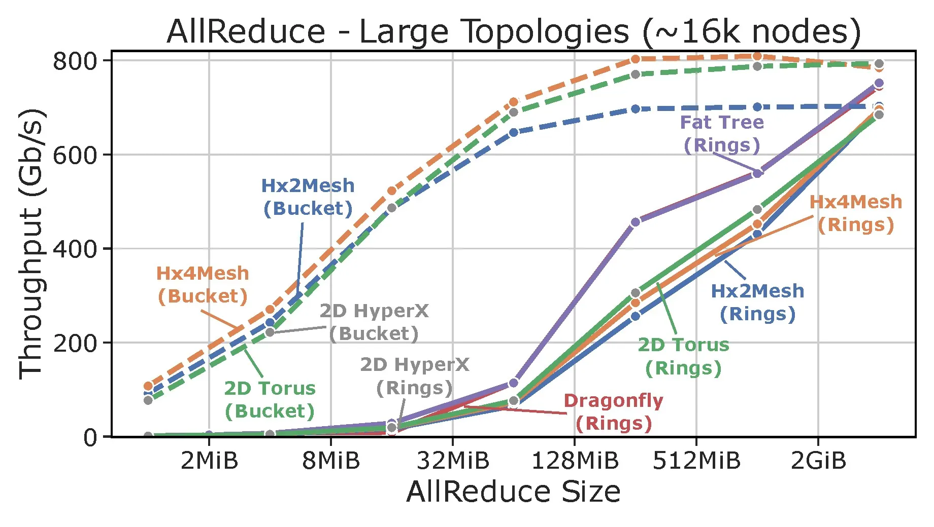
Full system allreduce job. This experiment shows a single job using the last two allreduce algorithms on various topologies. In Dragonfly and fat tree, each accelerator connects with a single NIC to each of the four planes and we use the standard “ring” algorithm. For the single allreduce on the large HxMesh clusters, we use both the two bidirectional rings (“rings”) as well as the bucket (“bucket”) algorithm. Figure 8 shows the achieved bandwidths.
We see that all topologies deliver nearly full bandwidth for the ring algorithms. For large messages, HxMesh is 2.8x to 14.5x cheaper per bandwidth than a nonblocking fat tree (Table 2). On networks with a Cartesian structure (HammingMesh, Torus, and HyperX) the bucket algorithm outperforms the ring algorithm at any message size. The only exception is for jobs where one of the two dimension is much smaller than the other, where the ring algorithm outperforms the bucket algorithm (not shown), highlighting the importance of using multi-algorithms to optimize performance, similar to established practice in MPI.25
4.2 DNN Workloads
We now proceed to define accurate communication patterns including computation times for real DNN models. For this, we choose four large representative models: ResNet-152, CosmoFlow, DLRM, and Transformers (GPT3) trained in FP32. We discuss only DLRM and Transformers, and a more detailed discussion covering the other models can be found in the full version of this paper.10 We use NVIDIA’s A100 GPU to benchmark runtimes of operators and we model communication times based on the data volumes.
4.2.1 Communication traffic characterization.
All example models are constructed of a sequence of identical layers containing multiple operators. Each parallel dimension carries a different volume, depending on the details of the model, training hyperparameters, and the other dimensions. We assume the most general case where the network can utilize all three forms of parallelism running on D × P × O accelerators.
Data dimension. If we only have data parallelism (O = P = 1), then each process needs to reduce all gradients. If we distribute the model between O or P dimension processes, then the total allreduce size is . The reduction happens once at the end of each iteration after processing a full minibatch and draining the pipeline. It can be overlapped per layer using nonblocking allreduce.13
Pipeline dimension. If we only have pipeline parallelism (D = O = 1) and NA output activations at the “cut” layer then each process sends all output values to the next process in the forward pass and the same volume of errors during the backward pass. If the layer and its inputs and outputs are distributed to O PEs, then the total send volume in this dimension is . This communication can be hidden at each accelerator as shown in Figure 9 by overlapping nonblocking send/receive operations (bottom, blue) with operator computation (top, green).
Operator dimension. For operator parallelism, each process’ send volume depends only on the operator parallelization itself and is not influenced by either D or P. The operator can be seen as the “innermost loop” in this sense. Each operator distribution scheme will have its own characteristics that we capture by VO = WNO. The operator communication volume during each forward and backward pass is a function of the local minibatch size M/DP per process.
4.2.2 DLRM.
DLRM20 uses a combination of model parallelism and data parallelism for its embedding and MLP layers, respectively. Two alltoall operations aggregate sparse embedding lookups in the forward pass, and their corresponding gradients in backward pass. Allreduce is required to synchronize the gradients of the data-parallel MLP layers. The parallelism of DLRM is limited by both the mini-batch size and the embedding dimension. DLRM is trained with up to 128 GPU nodes. The total runtimes on the fat tree variants are 2.96 ms, 2.97 ms, and 2.99 ms, respectively. On torus, the code executes for 3.12 ms. HyperX is at 2.94 ms. Hx2Mesh and Hx4Mesh are at 2.97 ms and 3.00 ms, respectively. On A100, DLRM computes around 95 us, 209 us, and 796 us for the embedding, feature interaction, and MLP layers respectively, and communicates 1 MB per alltoall and 2.96 MB per allreduce.
4.2.3 Transformers
Transformers are the most communication intensive.14 A transformer block consists of multi-head attention (MHA) and two feed-forward (FF) layers. The MHA and FF input/outputs are of size (embedding dimension×batch×sequence length). For example, GPT-3’s7 feed forward layers multiply 49,152×12,288 with 12,288×2,048 matrices per example in each layer.
GPT-3 has a total of 96 layers and each layer has activations of size NA = 4 · 2,048 × 12, 288 ≈ 100MB per example as input and output. We choose P = 96, such that each pipeline stage processes one layer, and no data parallelism (D = 1). For operator parallelism, we use O = 4 and the scheme outlined by Megatron-LM,24 which performs one allreduce for FF and one for MHA in both the forward and backward passes.
All operations are the same size as the layer input/output. Thus, the volume for both pipeline communication and operator-dimension allreduce is NA per example for forward and backward passes. One iteration of GPT-3 computes for 31.8ms. The total runtimes on the three fat tree variants are 34.8ms, 36.4ms, and 37.5ms, respectively. On torus, the code executes for 72.2 ms per iteration. HyperX is at 40.9ms. Hx2 and Hx4Mesh are at 41.7ms and 49.9ms, respectively.
For GPT-3 with Mixture-of-Experts (MoEs),18 we use 16 experts. In GPT-3, the FFs have 1.8B parameters. Therefore, each expert has 1.8B/16 ≈ 113M parameters. MoEs perform two alltoalls for FF in both the forward and backward passes, and all operations are the same size as the input/output. The computation time on an A100 is 49.9ms. The total runtime on the fat trees varies from 52.2ms to 52.9 ms depending on tapering. On torus, the code executes for 73.8ms per iteration. HyperX takes 53.9ms while Hx2 and Hx4Mesh are at 58.3ms and 63.3ms, respectively.
Figure 10 shows the relative cost savings of HxMesh compared to other topologies. These are calculated as the ratio of the network costs in Section 2 times the inverse of the ratio of communication overheads presented in this section.
We conclude that both Hx2 and Hx4Mesh significantly reduce network costs for DNN workloads. While some torus network configurations can be cheaper than Hx2Mesh, they provide significantly less allocation and management flexibility, especially in the presence of failures. Moreover, we also conclude that even in the presence of alltoall communications patterns in GPT-3 MoE and DLRM HxMesh topologies still offer a significant cost advantage compared to traditional topologies. As the scale of the network increases, Hx4Mesh becomes significantly more cost efficient than Hx2Mesh especially in the presence of alltoall traffic.
Discussion: We cover all additional related work and comparisons to other topologies, as well as significantly more detail on HammingMesh configuration options, tapering, diameter, cost, routing and deadlock avoidance, as well as scheduling with and without board failures in the full version of this paper.10
5 Conclusions
HammingMesh is optimized specifically for machine learning workloads and their communication patterns. It relies on the observation that deep learning training uses three-dimensional communication patterns and rarely needs global bandwidth. It supports extreme local bandwidth while controlling the cost of global bandwidth. It banks on an inexpensive local PCB-mesh interconnect together with a workload-optimized global connectivity forming virtual torus networks at adjustable global bandwidth.
Due to the lower number of switches and external cables, it can be nearly always more cost effective than torus networks while also offering higher global bandwidth and significantly higher flexibility in job allocation and dealing with failures.
All-in-all, we believe that HammingMesh will drive future deep learning systems and will also support adjacent workloads, such as (multi)linear algebra, quantum simulation, or parallel solvers, that have Cartesian communication patterns.
6 Acknowledgment
We thank Microsoft for hosting TH’s sabbatical where much of the idea was developed.11,12 We thank the whole Azure Hardware Architecture team and especially Doug Burger for their continued support and deep technical discussions. We thank the Swiss National Supercomputing Center (CSCS) for the compute resources on Piz Daint and the Slim Fly cluster (thanks to Hussein Harake) to run the simulations. Daniele De Sensi is supported by an ETH Post-doctoral Fellowship (19-2 FEL-50).




Join the Discussion (0)
Become a Member or Sign In to Post a Comment