
We introduce the heat method for solving the single- or multiple-source shortest path problem on both flat and curved domains. A key insight is that distance computation can be split into two stages: first find the direction along which distance is increasing, then compute the distance itself. The heat method is robust, efficient, and simple to implement since it is based on solving a pair of standard sparse linear systems. These systems can be factored once and subsequently solved in near-linear time, substantially reducing amortized cost. Real-world performance is an order of magnitude faster than state-of-the-art methods, while maintaining a comparable level of accuracy. The method can be applied in any dimension, and on any domain that admits a gradient and inner product—including regular grids, triangle meshes, and point clouds. Numerical evidence indicates that the method converges to the exact distance in the limit of refinement; we also explore smoothed approximations of distance suitable for applications where greater regularity is desired.
1. Introduction
The multiple-source shortest path problem seeks the distance from each point of a domain to the closest point within a given subset; different versions of this problem are fundamental to a wide array of problems across computer science and computational mathematics. Solutions date back at least to Dantzig’s work on linear programs35; typically the problem is formulated in terms of a weighted graph, as in Dijkstra’s algorithm. Often, however, one wishes to capture the distance on a continuous domain; a key example is illustrated in Figure 1 (left) where the graph distance will overestimate the straight-line Euclidean distance, no matter how fine the grid becomes. In 2D, an important development was the formulation of “exact” algorithms, where paths can cut through the faces of a triangulation8, 27; a great deal of subsequent work has focused on making these O(n2) algorithms practical for large datasets.40,46 However, for problems in data analysis and scientific computing it is not clear that the cost and complexity of exact algorithms are always well-justified, since the triangulation itself is only an approximation of the true domain (see Figure 4).

Figure 1. In contrast to algorithms that compute shortest paths along a graph (left), the heat method computes the distance to points on a continuous, curved domain (right). A key advantage of this method is that it is based on sparse linear equations that can be efficiently prefactored, leading to dramatically reduced amortized cost.
A very different approach is to formulate the problem in terms of partial differential equations (PDEs), where domain approximation error can be understood via, for example, traditional finite element analysis. However, the particular choice of continuous formulation has a substantial impact on computation. The heat method was inspired by S.R.S. Varadhan’s classic result in differential geometry42 relating heat diffusion and geodesic distance, which measures the length along shortest and straightest curves through the domain rather than straight lines through space. Our key observation is that one can decompose distance computation into two stages: first determine the direction along which distance increases, then recover the distance itself. Moreover, since each stage amounts to a standard problem in numerical linear algebra, one can leverage existing algorithms and software to improve the efficiency and robustness of distance computation. Although this approach can in principle be used in the context of graph distance, its real utility lies in approximating the distance on continuous, curved domains. This approach has proven effective for a diverse range of applications in computational neuroscience, geometric modeling, medical imaging, computational design, and machine learning (Section 2), and has recently inspired more accurate variations of our original method.3

Imagine touching a scorching hot needle to a single point on a surface. Over time heat spreads out over the rest of the domain and can be described by a function kt,x(y) called the heat kernel, which measures the heat transferred from a source x to a destination y after time t. A well-known relationship between heat and distance is Varadhan’s formula,42 which says that the distance ϕ between any pair of points x, y on a curved domain can be recovered via a simple pointwise transformation of the heat kernel:

The intuition behind this behavior stems from the fact that heat diffusion can be modeled as a large collection of hot particles taking random walks starting at x: any particle that reaches a distant point y after a small time t has had little time to deviate from the shortest possible path. Previously, however, this relationship had not been exploited by numerical algorithms that compute distance.
Why had Varadhan’s formula been overlooked in this context? The main reason, perhaps, is that it requires a precise numerical reconstruction of the heat kernel, which is difficult to obtain—applying the formula to a mere approximation of kt,x does not yield the correct result, as illustrated in Figures 2 and 8. The heat method circumvents this issue by working with a broader class of inputs, namely any function whose gradient is parallel to the gradient of the true distance function. We can then separate computation into two stages: first find the gradient, then recover the distance itself.

Figure 2. Given an exact reconstruction of the heat kernel (top Left) Varadhan’s formula can be used to recover geodesic distance (bottom left) but fails in the presence of approximation or numerical error (middle, right), as shown here for a point source in 1D. The robustness of the heat method stems from the fact that it depends only on the direction of the gradient.
Relative to existing algorithms, the heat method offers two major advantages. First, it can be applied to virtually any type of geometric discretization, including regular grids, polygonal meshes, and point clouds. Second, it involves only sparse linear systems, which can be prefactored once and rapidly resolved many times—this feature substantially reduces the amortized cost for applications that require repeated distance queries on a fixed geometric domain. Moreover, because the heat method is built on standard linear PDEs that are widespread in scientific computing, it can immediately take advantage of new developments in numerical linear algebra and parallelization.

Figure 3. The heat method computes the shortest distance to a subset γ of a given domain. Gray curves indicate isolines of the distance function.
2. Related Work
The prevailing approach to distance computation is to solve the eikonal equation

subject to boundary conditions ϕ/γ = 0 over some subset γ of the domain (like a point or a curve). Intuitively, this equation says something very simple: as we move away from the source, the distance function ϕ must change at a rate of “one meter per meter.” Computationally, however, this formulation is nonlinear and hyperbolic, making it difficult to solve directly. Typically one applies an iterative relaxation scheme such as Gauss-Seidel—special update orders are known as fast marching and fast sweeping, which are some of the most popular algorithms for distance computation on regular grids37 and triangulated surfaces.19 These algorithms can also be used on implicit surfaces,25 point clouds,26 and polygon soup,7 but only indirectly: distance is computed on a simplicial mesh or regular grid that approximates the original domain. Implementation of fast marching on simplicial grids is challenging due to the need for nonobtuse triangulations (which are notoriously difficult to obtain) or else an iterative unfolding procedure that preserves monotonicity of the solution; moreover these issues are not well-studied in dimensions greater than two. Fast marching and fast sweeping have asymptotic complexity of O(n log n) and O(n), respectively, but sweeping is often slower due to the large number of sweeps required to obtain accurate results.16

Figure 4. Convergence of distance approximations on the unit sphere with respect to mean edge length; as a baseline for comparison, we use the analytical solution ϕ(x, y) = cos-1(x • y). Notice that even with a nice tessellation, the exact distance along the polyhedron converges only quadratically to the true distance along the sphere it approximates. (Linear and quadratic convergence are plotted as dashed lines for reference.)
One drawback of these methods is that they do not reuse information: the distance to different source sets γ must be computed entirely from scratch each time. Also note that both sweeping and marching present challenges for parallelization: priority queues are inherently serial, and irregular meshes lack a natural sweeping order.
In a different development, Mitchell et al.27 give an O(n2 log n) algorithm for computing the exact polyhedral distance from a single source to all other vertices of a triangulated surface. Surazhsky et al.40 demonstrate that this algorithm tends to run in sub-quadratic time in practice, and present an approximate O(n log n) version of the algorithm with guaranteed error bounds; Bommes and Kobbelt4 extend the algorithm to polygonal sources. Similar to fast marching, these algorithms propagate distance information in wavefront order using a priority queue, again making them difficult to parallelize. More importantly, the amortized cost of these algorithms (over many different source subsets γ) is substantially greater than for the heat method since they do not reuse information from one subset to the next. Finally, although40 greatly simplifies the original formulation, these algorithms remain challenging to implement and do not immediately generalize to domains other than triangle meshes.

Figure 5. The heat method has been applied to a diverse range of tasks that demand repeated geodesic distance queries. Here, geodesic distance drives a differential growth model (left) that is used for computational design (right). Images courtesy Nervous System/Jesse Louis-Rosenberg.
Closest to our approach is the recent method of Rangarajan and Gurumoorthy,32 who do not appear to be aware of Varadahn’s formula—they instead derive an analogous relationship between the distance function and solutions ψ to the time-independent Schrödinger equation; this derivation applies only in flat Euclidean space rather than general curved domains. Moreover, they compute solutions using the fast Fourier transform, which limits computation to regular grids.
A slight modification of the heat method allows us to compute a smoothed distance function, useful in contexts where sharp discontinuities can cause subsequent numerical difficulties. Previous smooth distance approximations provide this regularity at the cost of poor approximation of the true geometric length10, 14, 21, 33; see Section 3.3 for a comparison.

Figure 6. The three steps of the heat method. (I) Heat u is allowed to diffuse for a brief period of time (left). (II) The temperature gradient ∇u (center left) is normalized and negated to get a unit vector field X (center right) pointing along geodesics. (III) A function ϕ whose gradient follows X recovers the final distance (right).
Recently, the heat method has facilitated a variety of tasks in computational science and data analysis. For example, Huth et al.15 use fast distance queries to optimize a probabilistic model of cortical organization; van Pelt et al.41 use the heat method to assist cerebral aneurysm assessment; Zou et al.47 use the heat method for efficient tool path planning; Solomon et al.38 leverage our approach to efficiently solve optimal transport problems on geometric domains; Lin et al.20 apply this approach to vector-valued data in the context of manifold learning. Figure 5 shows a real-world design application of the heat method based on differential growth. Various improvements have also been made to the original algorithm; for instance, de Goes et al.13 and Yang and Cohen45 describe two different ways to extend the method to accurate computation of anisotropic distance; it has also been adapted to voxelizations6, C1 finite elements,29 and subdivision surfaces.12 Finally, Belyaev and Fayolle3 provide a variational interpretation of our method, observing that more accurate results can be obtained by either iterating the heat method, or by applying more sophisticated descent strategies.
3. The Heat Method
A useful feature of the heat method is that the basic algorithm can be described in the purely continuous setting (i.e., in terms of curved surfaces, or more generally, smooth manifolds) rather than in terms of discrete data structures and algorithms. In other words, at this point one should not imagine that we have chosen a particular data structure (triangle meshes, grids, point clouds, etc.) or even dimension (2D, 3D, etc.). Instead, we focus on a general principle that can be applied on many different domains in different dimensions. We will later explore several particular choices of spatial and temporal discretization (Sections 3.1 and 3.2); further alternatives have been explored in recent literature.13, 29, 45

Figure 7. Distance to the boundary on a region in the plane (left) or a surface in space (right) is achieved by simply placing heat along the boundary curve.
In general, the heat method can be applied in any setting where one has a gradient operator ∇, divergence operator ∇, and Laplace operator Δ = ∇ · ∇—standard derivatives from vector calculus, possibly generalized to curved domains. Expressed in terms of these operators, the heat method consists of three basic steps:

The function ϕ approximates the distance to a given source set, approaching the true distance as t goes to zero (Equation 1). For instance, to recover the distance to a single point x we use initial conditions u0 = δ(x), that is, a Dirac delta encoding an “infinite spike” of heat. More generally we can obtain the distance to any subset γ by letting u0 be a generalized Dirac distribution42—essentially an indicator function over γ; see Figures 3 and 7. Note that since the solution to (III) is determined only up to an additive constant, final values are shifted such that the smallest distance is zero.
The heat method can be motivated as follows. Consider an approximation ut of heat flow for a fixed time t. Unless ut exhibits precisely the right rate of decay, Varadhan’s transformation
 will yield a poor approximation of the true geodesic distance ϕ because it is highly sensitive to errors in magnitude (see Figures 2 and 8). The heat method asks for something different: it requires only that the gradient ∇ut point in the right direction, that is, parallel to ∇ϕ. Magnitude can safely be ignored since we know (from the eikonal equation) that the gradient of the true distance function has unit length. We therefore compute the normalized gradient field X = − ∇ut/|∇ut| and find the closest scalar potential ϕ by minimizing
 , or equivalently, by solving the corresponding Euler-Lagrange equations Δϕ = ∇ · X.36 The overall procedure is depicted in Figure 6.

Figure 8. Left: Varadhan’s formula. Right; the heat method. Even for very small values of t, simply applying Varadhan’s formula does not provide an accurate approximation of geodesic distance (top left); for large values of t spacing becomes even more uneven (bottom left). Normalizing the gradient results in a more accurate solution, as indicated by evenly spaced isolines (top right), and is also valuable when constructing a smoothed distance function (bottom right).
This procedure is used as the starting point for a family of discrete algorithms, as outlined in Sections 3.1–3.3. Note that some details have been omitted from this manuscript, and can be found in Crane et al.11
To translate our continuous procedure (Algorithm 1) into a discrete algorithm, we must replace derivatives in space and time with suitable approximations. The heat equation from step I of Algorithm 1 can be discretized in time using a single backward Euler step for some fixed time t—in practice, this means we simply solve the linear equation

over the entire domain M, where id denotes the identity operator. Note that at this point we still have not discretized space; spatial discretization is discussed in Section 3.2. We can get a better understanding of solutions to Equation (3) by considering the elliptic boundary value problem

which for a point source yields a solution νt equal to ut up to a multiplicative constant. As established by Varadhan in his proof of Equation (1), νt also has a close relationship with distance, namely

This relationship ensures the validity of steps II and III since the transformation applied to νt preserves the direction of the gradient.
Here we detail several possible implementations of the heat method on triangle meshes, polygon meshes, and point clouds. Note that the heat method can also be used on flat Euclidean domains of any dimension by simply applying standard finite differences on a regular grid; Belyaev and Fayolle3 outline implementation on tetrahedral (3D) meshes.

Figure 9. Since the heat method is based on well-established discrete operators like the Laplacian, it is easy to adapt to a variety of geometric domains. Above: distance on a hippo composed of high-degree nonplanar (and sometimes nonconvex) polygonal faces.
Triangle meshes. Let u ∈ ℝ|v| specify a piecewise linear function on a triangulated surface with vertices V, edges E, and faces F. A standard discretization of the Laplacian at a vertex i is given by

where Ai is one third the area of all triangles incident on vertex i, the sum is taken over all neighboring vertices j, and αβij, βij are the angles opposing the corresponding edge.23 We can express this operation via a matrix L = M-1LC, where M ∈ ℝ|v|×|v| is a diagonal matrix containing the vertex areas and LC ∈ ℝ|v|×|v| is the cotan operator representing the remaining sum. Heat flow can then be computed by solving the symmetric positive-definite system

where δγ is a Kronecker delta (or indicator function) over γ. The gradient in a given triangle can be expressed succinctly as

where Af is the area of the triangle, N is its outward unit normal, ei is the ith edge vector (oriented counter-clockwise), and ui is the value of u at the opposing vertex. The integrated divergence associated with vertex i can be written as

where the sum is taken over incident triangles j each with a vector Xj, e1, and e2 are the two edge vectors of triangle j containing i, and θ1, θ2 are the opposing angles. If we let b ∈ ℝ|v be the vector of (integrated) divergences of the normalized vector field X, then the final distance function is computed by solving the symmetric Poisson problem

As noted in Section 3.1, the solution to step I is a function that decays exponentially with distance. Fortunately, normalization of small values is not a problem because floating point division involves only arithmetic on integer exponents; likewise, the large range of magnitudes does not adversely affect accuracy because gradient calculation is local. For the calculation of phi itself we advocate the use of a direct (Cholesky) solver in double precision; empirically we observe roughly uniform pointwise relative error across the domain.

Figure 10. The heat method can be applied directly to scattered point clouds. Left: face scan with holes and noise. Right: kitten surface with connectivity removed. Yellow points are close to the source.
Polygon meshes. Curved surfaces are often described by polygons that are neither planar nor convex; although such polygons can of course be triangulated, doing so can adversely affect an existing computational pipeline. We instead leverage the polygonal Laplacian of Alexa and Wardetzky1 to implement the heat method directly on polygonal meshes—the only challenge in this setting is that for nonplanar polygons the gradient vector no longer has a clear geometric meaning. This issue is resolved by noting that we need only the magnitude |∇u| of the gradient; see Crane et al,11 Section 3.2.2 for further details. Figure 9 demonstrates distance computed on an irregular polygonal mesh.
Point clouds. Raw geometric data is often represented as a discrete point sample P ⊂ ℝn of some smooth surface M. Rather than convert this data into a polygon mesh, we can directly implement the heat method using the point cloud Laplacian of Liu et al.,22 which extends previous work by Belkin et al.2 Computation of the gradient and divergence are described by Crane et al,11 Section 3.2.3. Other discretizations are certainly possible (see for instance the work of Luo et al.23); we picked one that was simple to implement in any dimension. It is particularly interesting to note that the cost of the heat method depends primarily on the intrinsic dimension n of M, whereas methods based on fast marching require a grid of the same dimension m as the ambient space25—this distinction is especially important in contexts like machine learning where m may be significantly larger than n.
Choice of time step. Accuracy of the heat method relies in part on the time step t. In the smooth setting, Equation (5) suggests that smaller values of t yield better approximations of geodesic distance. In the discrete setting we instead observe the somewhat surprising behavior that the limit solution to Equation (3) depends only on the number of edges between a pair of vertices, independent of how we might try to incorporate edge lengths into our formulation—see Crane et al.,11 Appendix A. Therefore, on a fixed mesh decreasing the value of t does not necessarily improve accuracy, even in exact arithmetic—to improve accuracy we must simultaneously refine the mesh and decrease t accordingly. Moreover, very large values of t produce an over-smoothed approximation of geodesic distance (Section 3.3). For a fixed mesh, we therefore seek an optimal time step t* that is neither too large nor too small.

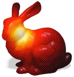
Figure 11. A source on the front of the Stanford Bunny results in nonsmooth cusps on the opposite side. By running heat flow for progressively longer durations t, we obtain smoothed approximations of geodesic distance (right).
An optimal value of t* is difficult to obtain due to the complexity of analysis involving the cut locus.28 We instead use a simple estimate that works well in practice, namely t = mh2 where h is the mean spacing between adjacent nodes and m > 0 is a constant. This estimate is motivated by the fact that h2ϕ is invariant with respect to scale and refinement; numerical experiments suggest that m = 1 yields near-optimal accuracy for a wide variety of problems. In this paper the time step

is therefore used uniformly throughout all tests and examples, except where we explicitly seek a smoothed approximation of distance, as in Section 3.3. For highly nonuniform meshes one could set h to the maximum spacing, providing a more conservative estimate. Numerical underflow could theoretically occur for extremely small t, though we do not encounter this issue in practice.

Figure 12. Top row: our smoothed approximation of geodesic distance (left) and biharmonic distance (center) both mitigate sharp “cusps” found in the exact distance (right), yet our approximation provides more even spacing of isocontours. Bottom row: biharmonic distance (center) tends to exhibit elliptical level lines near the source, while our smoothed distance (left) maintains isotropic circular profiles as seen in the exact distance (right).
Numerics. As demonstrated in Figures 10, 18, and 19, one does not need a particularly nice mesh or point cloud to get a reasonable distance function. However, as with any numerical method, accuracy and other properties of the solution may be influenced by the quality of the mesh. For instance, in some applications one may wish to avoid “spurious minima,” that is, local maxima or minima that do not appear in the true (smooth) distance function. At present, there is no numerical scheme that guarantees the absence of spurious minima on arbitrary meshes, including exact polyhedral schemes.17 Empirically, however, we observe that the heat method produces fewer spurious minima than either fast marching or the biharmonic distance (see Figure 20), in part due to regularization from the Hodge step (step III). In cases where one wishes to avoid spurious minima altogether, we advocate the use of Delaunay meshes.
Geodesic distance fails to be smooth at points in the cut locus, that is, points at which there is no unique shortest path to the source—these points appear as sharp cusps in the level lines of the distance function. Non-smoothness can result in numerical difficulty for applications which need to take derivatives of the distance function ϕ (e.g., level set methods), or may simply be undesirable aesthetically.

Figure 13. Effect of Neumann (top-left), Dirichlet (top-right) and averaged (bottom-left) boundary conditions on smoothed distance. Averaged boundary conditions mimic the behavior of the same surface without boundary.
Several distances have been designed with smoothness in mind, including diffusion distance,10 commute-time distance,14 and biharmonic distance21 (see the last reference for a more detailed discussion). These distances satisfy a number of important properties (smoothness, isometry-invariance, etc.), but are poor approximations of true geodesic distance, as indicated by uneven spacing of isolines (see Figure 12, middle). They can also be expensive to evaluate, requiring one to either solve a linear system for each vertex, or compute a large number of eigenvectors of the Laplace matrix (∼150 to 200 in practice).

Figure 14. For path planning, the behavior of geodesics can be controlled via boundary conditions and the time step t. Top-left: Neumann conditions encourage boundary adhesion. Top-right: Dirichlet conditions encourage avoidance. Bottom-left: small values of t yield standard straight-line geodesics. Bottom-right: large values of t yield more natural trajectories.
In contrast, one can rapidly construct smoothed approximations of geodesic distance by simply applying the heat method for large values of t (Figure 11). The computational cost remains the same, and isolines are evenly spaced for any value of t due to normalization (step II); the solution is isometry invariant since it depends only on intrinsic operators. For a time step t = mh2, meaningful values of m are found in the range 1 – 106—past this point the term tϕ dominates, resulting in little visible change.
To solve the equations in steps I and II, we must define the behavior of derivatives near the boundary. Intuitively, the behavior of our distance approximation should not be significantly influenced by the shape of the boundary (Figure 13)—for instance, cutting off a corner of a convex domain should not affect the distance at the points that remain. For exact distance computation, we can apply standard zero-Neumann or zero-Dirichlet boundary conditions, since this choice does not affect the behavior of the smooth limit solution (see Renesse44 Corollary 2 and Norri,30 Theorem 1.1, respectively). Boundary conditions do however alter the behavior of our smoothed distance. Although there is no well-defined “correct” behavior for this smoothed function, we advocate the use of boundary conditions obtained by taking the mean of the Neumann solution uN and the Dirichlet solution uD, that is,
 . The intuition behind this behavior again stems from a random walker interpretation: zero Dirichlet conditions absorb heat, causing walkers to “fall off” the edge of the domain. Neumann conditions prevent heat from flowing out of the domain, effectively “reflecting” random walkers. Averaged conditions mimic the behavior of a domain without boundary: the number of walkers leaving equals the number of walkers returning. Figure 14 shows how boundary conditions affect the behavior of geodesics in a path-planning scenario.

4. Evaluation
A key advantage of the heat method is that the linear systems in steps I and III can be prefactored. Our implementation uses sparse Cholesky factorization,9 which for Poisson-type problems has guaranteed sub-quadratic complexity but in practice scales much better5; moreover there is strong evidence to suggest that sparse systems arising from elliptic PDEs can be solved in very close to linear time.34, 39 Independent of these issues, the amortized cost for problems with a large number of right-hand sides is roughly linear, since back substitution can be applied in essentially linear time. See inset for a breakdown of relative costs in our implementation; Potential is the time taken to compute the right hand side in step III.

Table 1. Comparison with fast marching and exact polyhedral distance
In practice, a number of factors affect the run time of the heat method including the choice of spatial discretization, discrete Laplacian, and geometric data structures. As a typical example, we compared the scheme from Triangle meshes section to the first-order fast marching method of Kimmel and Sethian19 and the exact algorithm of Mitchell et al.,27 using the state-of-the-art fast marching implementation of Peyré and Cohen31 and the exact implementation of Kirsanov.40 The heat method was implemented in ANSI C in double precision using a vertex-face adjacency list. Single-threaded performance was measured on a 2.4 GHz Intel Core 2 Duo (Table 1). Note that even for a single distance computation the heat method outperforms fast marching; more importantly, updating distance for new subsets γ is consistently an order of magnitude faster (or more) than both fast marching and the exact algorithm.

Figure 15. Meshes used in Table 1. Left to right: Bunny, Isis, Horse, Bimba, Aphrodite, Lion, Ramses.
We examined errors in the heat method, fast marching,19 and the polyhedral distance,27 relative to mean edge length h on triangulated surfaces. Both fast marching and the heat method appear to exhibit linear convergence; it is interesting to note that even the exact polyhedral distance provides only quadratic convergence. Keeping this fact in mind, Table 1 uses the polyhedral distance as a baseline for comparison on more complicated geometries—Max is the maximum error as a percentage of mesh diameter and Mean is the mean relative error at each vertex. Note that fast marching tends to achieve a smaller maximum error, whereas the heat method does better on average. Figure 16 gives a visual comparison of accuracy; the only notable discrepancy is a slight smoothing at sharp cusps, which may explain the larger maximum error. Figure 17 indicates that smoothing does not interfere with the extraction of the cut locus—here we visualize values of |Δϕ| above a fixed threshold. Overall, the heat method exhibits errors of the same order and magnitude as fast marching (at lower computational cost) and is therefore suitable in applications where fast marching is presently used; see Crane et al.11 for more extensive comparisons.

Figure 16. Visual comparison of accuracy. Left: exact polyhedral distance. Using default parameters, the heat method (middle) and fast marching (right) both produce results of comparable accuracy, here within less than 1% of the polyhedral distance—see Table 1 for a more detailed comparison.

Figure 17. Medial axis of the hiragana letter “a” extracted by thresholding second derivatives of the distance to the boundary. Left: fast marching. Right: heat method.
More recent implementations of the heat method improve accuracy by using a different spatial discretization,29 or by iteratively updating the solution.3 The accuracy of fast marching schemes is determined by the choice of update rule—a number of highly accurate rules have been developed for regular grids (e.g., HJ WENO18), but fewer options are available on irregular domains such as triangle meshes, the predominant choice being the first-order update of Kimmel and Sethian.19 Finally, the approximate algorithm of Surazhsky et al.40 provides an interesting comparison since it tends to produce results more accurate than fast marching at a similar computational cost. However, accuracy is measured relative to the polyhedral distance rather than the smooth geodesic distance of the approximated surface. Like fast marching, Surazhsky’s method does not take advantage of precomputation and therefore exhibits a significantly higher amortized cost than the heat method; it is also limited to triangle meshes.

Figure 18. Smoothed geodesic distance on an extremely poor triangulation with significant noise—note that small holes are essentially ignored. Also note good approximation of distance even along thin slivers in the nose.

Figure 19. Tests of robustness. Left: our smoothed distance (m = 104) appears similar on meshes of different resolution. Right: even for meshes with severe noise (top) we recover a good approximation of the distance function on the original surface (bottom, visualized on noise-free mesh).

Figure 20. In any method based on a finite element approximation, mesh quality will affect the quality of the solution. However, because the heat method is based on solving low-order elliptic equations (rather than high-order or hyperbolic equations), it often produces fewer numerical artifacts. Here, for instance, we highlight spurious extrema in the distance function (i.e., local maxima and minima) produced by the fast marching method (left), biharmonic distance (middle), and the heat method (right) on an acute Delaunay mesh (top) and a badly degenerate mesh (bottom). Inset figures show closeup view of isolines for the bottom figure.
Two factors contribute to the robustness of the heat method, namely (1) the use of an unconditionally stable time discretization and (2) an elliptic rather than hyperbolic formulation (i.e., relatively stable local averaging vs. more sensitive global wavefront propagation). Figure 19 verifies that the heat method continues to work well even on meshes that are poorly discretized or corrupted by a large amount of noise (here modeled as uniform Gaussian noise applied to the vertex coordinates). In this case we use a moderately large value of t to investigate the behavior of our smoothed distance; similar behavior is observed for small t values. Figure 18 illustrates the robustness of the method on a surface with many small holes as well as long sliver triangles.
5. Conclusion
The heat method is a simple, general method that can be easily incorporated into a broad class of algorithms. However, a great deal remains to be explored, including further investigation of alternative spatial discretizations, and formal analysis of convergence under refinement. Further exploration of the parameter t also provides an avenue for future work (especially in the case of variable spacing), though one should note that the existing estimate already outperforms fast marching in terms of mean error (Table 1). Another natural question is whether a similar transformation can be applied to a larger class of Hamilton-Jacobi equations; it is likewise enticing to apply a similar principle to distance computation on domains that do not immediately resemble a continuous domain (such as a weighted graph).
Acknowledgments
This work was funded by a Google PhD Fellowship and a grant from the Fraunhofer Gesellschaft. Thanks to Michael Herrmann for inspiring discussions. Meshes are provided courtesy of the Stanford Computer Graphics Laboratory, the AIM@Shape Repository, Luxology LLC, and Jotero GbR (http://www.evolution-of-genius.de/).


Join the Discussion (0)
Become a Member or Sign In to Post a Comment