Abstract
The paper discusses algorithmic priority inversion in mission-critical machine inference pipelines used in modern neural-network-based perception subsystems and describes a
solution to mitigate its effect. In general, priority inversion occurs in computing systems when computations that are “less important” are performed together with or ahead of those that are “more important.” Significant priority inversion occurs in existing machine inference pipelines when they do not differentiate between critical and less critical data. We describe a framework to resolve this problem and demonstrate that it improves a perception system’s ability to react to critical inputs, while at the same time reducing platform cost.
1. Introduction
Algorithmic priority inversion plagues modern mission-critical machine inference pipelines such as those implementing perception modules in autonomous drones and self-driving cars. We describe an initial solution for removing such priority inversion from neural-network-based perception systems. This research was originally published in RTSS 2020.17 While it is evaluated in the context of autonomous driving only, the design principles described below are expected to remain applicable in other contexts.
The application of artificial intelligence (AI) has revolutionized cyber-physical systems but has posed novel challenges in aligning computational resource consumption with mission-specific priority. Perception is one of the key components that enable system autonomy. It is also a major efficiency bottleneck that accounts for a considerable fraction of resource consumption.3,12 In general, priority inversion occurs in computing systems when computations that are less critical (or that have longer deadlines) are performed together with or ahead of those that are more critical (or that have shorter deadlines). Current neural-network-based machine intelligence software suffers from a significant form of priority inversion on the path from perception to decision-making, because it processes input data sequentially in arrival order as opposed to processing important parts of a scene first. By resolving this problem, we significantly improve the system’s responsiveness to critical inputs at a lower platform cost. The work applies to intelligent systems that perceive their environment in real-time (using neural networks), such as self-driving vehicles,1 autonomous delivery drones,5 military defense systems,2 and socially-assistive robotics.8
To understand the present gap, observe that current deep perception networks perform many layers of manipulation of large multidimensional matrices (called tensors). The underlying neural network libraries (e.g., TensorFlow) are reminiscent of what used to be called the cyclic executive4 in early operating system literature. Cyclic executives, in contrast to priority-based scheduling,11 processed all pieces of incoming data at the same priority and fidelity (e.g., as nested loops). Given incoming data frames (e.g., multicolor images or 3D LiDAR point clouds), modern neural network algorithms process all data rows and columns at the same priority and fidelity. Importance cues drive attention weights in AI computations, but not actual computational resource assignments.
This flat processing is in sharp contrast to the way humans process information. Human cognitive perception systems are good at partitioning the perceived scene into semantically meaningful partial regions in real-time, before allocating different degrees of attention (i.e., processing fidelity) and prioritizing the processing of important parts, to better utilize the limited cognitive resources. Given a complex scene, such as a freeway with multiple nearby vehicles, human drivers are good at understanding what to focus on to plan a valid path forward. In fact, human cognitive capacity is not sufficient to simultaneously absorb everything in their field of view. For example, if faced with an iMax screen partitioned into a dozen subdivisions, each playing an independent movie, humans would be fundamentally incapable of giving all such simultaneously playing movies sufficient attention. This suggests that GPUs that can, in fact, keep up with processing all pixels of the input scene are fundamentally and needlessly over-provisioned. They could be substantially smaller if endowed with a human-like capacity to focus on part of the scene only. The lack of prioritized allocation of processing resources to different parts of an input data stream (e.g., from a camera) is an instance of algorithmic priority inversion. As exemplified above, it results in significant resource waste, processing less important stimuli together with more important ones. To avoid wasting resources, the architecture described in this paper allows machine perception pipelines to partition the scene into regions of different criticality, prioritize the processing of important parts ahead of others, and provide higher processing fidelity on critical regions.
2. System Architecture
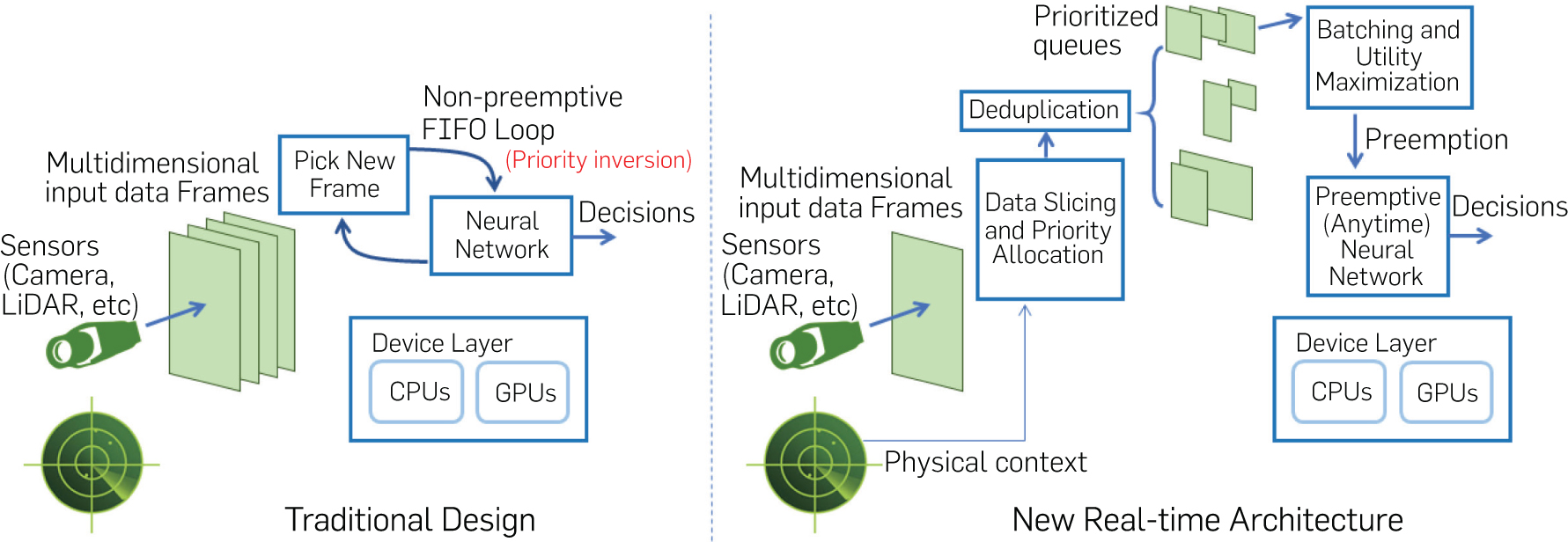
Consider a simple pipeline composed of a camera that observes its physical environment, a neural network that processes the sampled frames, and a control unit that must react in real-time. Figure 1 contrasts the traditional design of such a machine inference pipeline to the proposed architecture. In the traditional design, the captured input data frames are processed sequentially by the neural network without preemption in execution.
Unfortunately, the multi-dimensional data frames captured by modern sensors (e.g., colored camera images and 3D LiDAR point clouds) carry information of different degrees of criticality in every framea. Data of different criticality may require a different processing latency. For example, processing parts of the image that represent faraway objects does not need to happen every frame, whereas processing nearby objects, such as a vehicle in front, needs to be done immediately because of their impact on immediate path planning. To accommodate these differences in input data criticality, our machine perception pipeline breaks the input frame processing into four steps:
Data slicing and priority allocation: This module breaks up newly arriving frames into smaller regions of different degrees of criticality based on simple heuristics (i.e., distance-based criticality).
Deduplication: This module drops redundant regions (i.e., ones that refer to the same physical objects) across successive arriving frames.
“Anytime” neural network: This neural network implements an imprecise computation model that allows execution to be preempted while yielding partial utility from the partially completed computation. The approach allows newly arriving critical data to preempt the processing of less critical data from older frames.
Batching and utility maximization: This module sits between the data slicing and deduplication modules on one end and the neural network on the other. With data regions broken by priority, it decides which regions to pass to the neural network for processing. Since multiple regions may be queued for processing, it also decides how best to benefit from batching (that improves processing efficiency).
We refer to the subsystem shown in Figure 1 as the observer. The goal is to allow the observer to respond to more urgent stimuli ahead of less urgent ones. To make the observer concrete, we consider a video processing pipeline, where the input video frames get broken into regions of different criticality according to the distance information obtained from a ranging sensor (i.e., LiDAR). Different deadline-driven priorities are then assigned to the processing of these regions. We adopt an imprecise computation model for neural networks21 to achieve a hierarchy of different processing fidelities. We further introduce a utility-optimizing scheduling algorithm for the resulting real-time workload to meet deadlines while maximizing a notion of global utility (to the mission). We implement the architecture on an NVIDIA Jetson Xavier platform and do a performance evaluation on the platform using real video traces collected from autonomous vehicles. The results show that the new algorithms significantly improve the average quality of machine inference, while nearly eliminating deadline misses, compared to a set of state-of-the-art baselines executed on the same hardware under the same frame rate.
For completeness, below we first describe all components of the observer, respectively. We then detail the batching and utility maximization algorithm used.
2.1. Data slicing and priority allocation
This module breaks up input data frames into regions that require different degrees of attention. Objects with a smaller time-to-collision18 should receive attention more urgently and be processed at a higher fidelity. We further assume that the observer is equipped with a ranging sensor. For example, in autonomous driving systems, a LiDAR sensor measures distances between the vehicle and other objects. LiDAR point cloud-based object localization techniques have been proposed6 that provide a fast (i.e., over 200Hz) and accurate ranging and object localization capability. The computed object locations can then be projected onto the image obtained from the camera, allowing the extraction of regions (subareas of the image) that represent these localized objects, sorted by distance from the observer. For simplicity, we restrict those subareas to rectangular regions or bounding boxes. We define the priority (of bounding boxes) by time-to-collision, given the trajectory of the observer and the location of the object. Computing the time-to-collision is a well-studied topic and is not our contribution.18
2.2. Deduplication
The deduplication module eliminates redundant bounding boxes. Since the same objects generally persist across many frames, the same bounding boxes will be identified in multiple frames. The set of bounding boxes pertaining to the same object in different frames is called a tubelet. Since the best information is usually the most recent, only the most recent bounding box in a tubelet needs to be acted on. The deduplication module identifies boxes with large overlaps as redundant and stores the most recent box only. For efficiency reasons described later, we quantize the used bounding box sizes. The deduplication module uses the same box size for the same object throughout the entire tubelet. Note that, in a traditional neural network processing pipeline, each frame is processed in its entirety before the next one arrives. Thus, no deduplication module is used. The option to add this time-saving module to our architecture arises because our pipeline can postpone the processing of some objects until a later time. By that time, updated images of the same object may arrive. This enables savings by looking at the latest image only when the neural network eventually gets around to processing the object.
2.3. The anytime neural network
A perfect anytime algorithm is one that can be terminated at any point, yielding utility that monotonically increases with the amount of processing performed. We approximate the optimal model with an imprecise computation model,14–16 where the processing consists of two parts: a mandatory part and multiple optional parts. The optional parts, or a portion thereof, can be skipped to conserve resources. When at least one optional part is skipped, the task is said to produce an imprecise result. Deep neural networks (e.g., image recognition models)10 are a concatenation of a large number of layers that can be divided into several stages, as we show in Figure 2. Ordinarily, an output layer is used at the end to convert features computed by earlier layers into the output value (e.g., an object classification). Prior work has shown, however, that other output layers can be forked off of intermediate stages producing meaningful albeit imprecise outputs based on features computed up to that point.20 Figure 3 shows the accuracy of ResNet-based classification applied to the ImageNet7 dataset at the intermediate stages of neural network processing. The quality of outputs increases when the network executes more optional parts. We set the utility proportionally to predictive confidence in result; a low confidence output is less useful than a high confidence output. The proportionality factor itself can be set depending on task criticality, such that uncertainty in the output of more critical tasks is penalized more.
2.4. Batching and utility maximization
This module decides the schedule of processing of all regions identified by the data slicing and prioritization module and that passes de-duplication. The data slicing module computes bounding boxes for objects detected, which constitute regions that require attention, each assigned a degree of criticality. The deduplication module groups boxes related to the same object into a tubelet. Only the latest box in the tubelet is kept. Each physical object gives rise to a separate neural network task to be scheduled. The input of that task is the bounding box for the corresponding object (cropped from the full scene).
3. The Scheduling Problem
In this section, we describe our task execution model, formulate the studied scheduling problem, and derive a near-optimal solution.
3.1. The execution model
As alluded to earlier, the scheduled tasks in our system constitute the execution of multi-layer deep neural networks (e.g., ResNet,10 as shown in Figure 2), each processing a different input data region (i.e., a bounding box). As shown in Figure 2, tasks are broken into stages, where each stage includes multiple neural network layers. The unit of scheduling is a single stage, whose execution is non-preemptive, but tasks can be preempted on stage boundaries. A task arrives when a new object is detected by the ranging sensor (e.g., LiDAR) giving rise to a corresponding new bounding box in the camera scene. Let the arrival time of task τi be denoted by ai. A deadline di > ai, is assigned by the data slicing and priority assignment module denoting the time by which the task must be processed (e.g., the corresponding object classified). The data slicing and priority assignment module are invoked at frame arrival time. Therefore, both ai and di are a multiple of frame inter-arrival time, H. No task can be executed after its deadline. Future object sizes, arrival times, and deadlines are unknown, which makes the scheduling problem an online decision problem. A combination of two aspects makes this real-time scheduling problem interesting: batching and imprecise computations. We describe these aspects below.
Batching. Stages of the neural network, in our architecture, are executed on a low-end embedded GPU. While such GPUs feature parallel execution, most require that the same kernel be executed on all GPU cores. This means that we can process different images concurrently on the GPU as long as we run the same kernel on all GPU cores. We call such concurrent execution, batching. Running the same kernel on all GPU cores means that we can only batch image processing tasks if both of the following apply: (i) they are executing the same neural network stage, and (ii) they run on the same size inputs. The latter condition is because the processing of different bounding box sizes requires instantiating different GPU kernels. Batching is advantageous because it allows us to better utilize the parallel processing capacity of GPU. To increase batching opportunities, we limit the size of possible bounding boxes to a finite set of options. For a given bounding box size k, at most B(k) tasks (processing inputs) can be batched together before overloading the GPU capacity. We call it the batching limit for the corresponding input size.
Imprecise computations. Let the number of neural network stages for task τi be Li (different input sizes may have different numbers of stages). We call the first stage mandatory and call the remaining stages optional. Following a recently developed imprecise computation model for deep neural networks (DNN),21 tasks are written such that they can return an object classification result once the mandatory stage is executed. This result then improves with the execution of each optional stage. Earlier work presented an approach to estimate the expected confidence in the correctness of the results of future stages, ahead of executing these stages.22 This estimation offers a basis for assessing the utility of future task stage execution. We denote the utility of task τi after executing j ≤ Li stages by Ri,j, where Ri,j is set proportionately to the predicted confidence in correctness at the conclusion of stage j. Note that, the expected utility can be different among tasks (depending in part on input size), but it is computable, non-decreasing, and concave with respect to the network stage.22
We denote by 𝒯(t) the set of current tasks at time t. A task, τi, is called current at time t, if ai ≤ t < di, and the task has not yet completed its last stage, Li. For task τi of input size, k, the execution time of the j-th stage is denoted by , where b is the number of batched tasks during the stage execution.
3.2. Problem formulation
We next formulate a new scheduling problem, called BAtched Scheduling with Imprecise Computations (BASIC). The problem is simply to decide on the number of stages li ≤ Li to execute for each task τi and to schedule the batched execution of those task stages on the GPU such that the total utility, , of executed tasks is maximized, and batching constraints are met (i.e., all used GPU cores execute the same kernel at any given time, and that the batching limit is not exceeded). In summary:
The BASIC problem. With online task arrivals, the objective of the BASIC problem is to derive a schedule x to maximize the aggregate system utility. The schedule decides three outputs: task stage execution order on the GPU, number of stages to execute for each task, and task batching decisions. For each scheduling period t, we use xt(i, j) ɛ {0, 1} to denote whether the j-th stage of task τi is executed. Besides, we use P to denote a batch of tasks, where |P| denotes the number of tasks being batched. The mathematical formulation of the optimization problem is:
(1) (2) (3) (4)The following constraints should be satisfied: (1) Each neural network stage can only be executed once; (2) No task can be executed after its deadline; (3) The execution of different stages of the same task must satisfy their precedence constraints; and (4) Only tasks with the same (image size, network stage) can be batched, and the number of batched tasks can not exceed the batching constraint of their image size.
Only one batch (kernel) can be executed on the GPU at any time. However, multiple batches can be executed sequentially in one scheduling period, as long as the sum of their execution times does not exceed the period length, H.
3.3. An online scheduling framework
We derive an optimal dynamic programming-based solution for the BASIC scheduling problem and express its competitive ratio relative to a clairvoyant scheduler (that has full knowledge of all future task arrivals). We then derive a more efficient greedy algorithm that approximates the dynamic programming schedule. We define the clairvoyant scheduling problem as follows:
Given information about all future tasks, the clairvoyant scheduling problem seeks to maximize the aggregate utility obtained from (stages of) tasks that are completed before their deadlines. The maximum aggregate utility is OPT.
With no future information, an online scheduling algorithm that achieves a competitive ratio of c (i.e., a utility ) is called c-competitive. A lower bound on the competitive ratio for online scheduling algorithms was shown to be 1.618.9
Our scheduler is invoked upon frame arrivals, which is once every H unit of time. We thus call H the scheduling period. We assume that all task stage execution times are multiples of some basic time unit δ, thereby allowing us to express H by an integer value. We further call the problem of scheduling current tasks within the period between successive frame arrivals, the local scheduling problem:
Given the set of current tasks, 𝒯(t), within the scheduling period, t, the local BASIC problem seeks to maximize the total utility gained within this scheduling period only.
We proceed to show that an online scheduling algorithm that optimally solves the local scheduling problem within each period will have a good competitive ratio. Let L be the maximum number of stages in any task, and let B be the maximum batching size:
If during each scheduling period, the local BASIC problem for that period is solved optimally, then the resulting online scheduling algorithm is min{2 + L, 2B + 1}-competitive with respect to a clairvoyant algorithm.
When no imprecise computation is considered, the competitive ratio is further reduced to:
If each task is only one stage long, and if the online scheduling algorithm solved the local BASIC problem in each scheduling period optimally, then the online scheduling algorithm is 3-competitive with respect to a clairvoyant algorithm.
3.4. Local scheduling algorithms
In this section, we propose two algorithms to solve the local BASIC problem. The first is a dynamic programming-based algorithm that optimally solves it but may have a higher computational overhead. The second is a greedy algorithm that is computationally efficient but may not optimally solve the problem.
Local dynamic programming scheduling. Since we only consider batching together on the GPU tasks that execute the same kernel (i.e., same stage on the same size input), we need to partition the scheduling interval, H, into sub-intervals where the above constraint is met. The challenge is to find optimal partitioning. This question is broken into three steps:
Step 1: Given an amount of time, Tj,k ≤ H, what is the maximum utility attainable by scheduling the same stage, j, of tasks that process an input of size k? The answer here simply depends on the maximum number of tasks that we can batch during Tj,k without violating the batching limit. If the time allows for more than one batch, dynamic programming is used to optimally size the batches. Let the maximum attainable utility thus found be denoted by .
Step 2: Given an amount of time, Tk ≤ H, what is the maximum utility attainable by scheduling (any number of stages of) tasks that process an input of size k? Let us call this maximum utility . Dynamic programming is used to find the best way to break interval Tk into non-overlapping intervals Tj,k, for which the total sum of utilities, , is maximum.
Step 3: Given the scheduling interval, H, what is the maximum utility attainable by scheduling tasks of different input sizes? Let us call this maximum utility U*. Dynamic programming is used to find the best way to break interval H into non-overlapping intervals Tk, for which the total sum of utilities, , is maximum.
The resulting utility, U*, as well as the corresponding breakdown of the scheduling interval constitute the optimal solution. In essence, the solution breaks down the overall utility maximization problem into a utility maximization problem over time sub-intervals, where tasks process only a given input size. These sub-intervals are in turn broken into sub-intervals that process the same stage (and input size). The intuition is that the subintervals in question do not overlap. We pose an order preserving assumption on task marginal utilities with the same image size.
For two tasksandwith the same size, if for one neural network stage j, we have, then it also holds.
Thus, the choice of the best subset of tasks to execute remains the same regardless of which stage is considered. Below, we describe the algorithm in more detail.
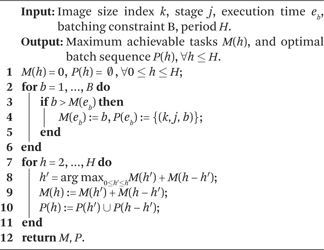
Step 1: For each object size k and stage j, we can use a dynamic programming algorithm to decide the maximum number of tasks M that can execute stage j in time 0 < Tj,k ≤ H. Observe that this computation can be done offline. The details are shown in Algorithm 1. With the optimal number, M, computed for each, is simply the sum of utilities of the M highest-utility tasks that are ready to execute stage j on an input of size k.
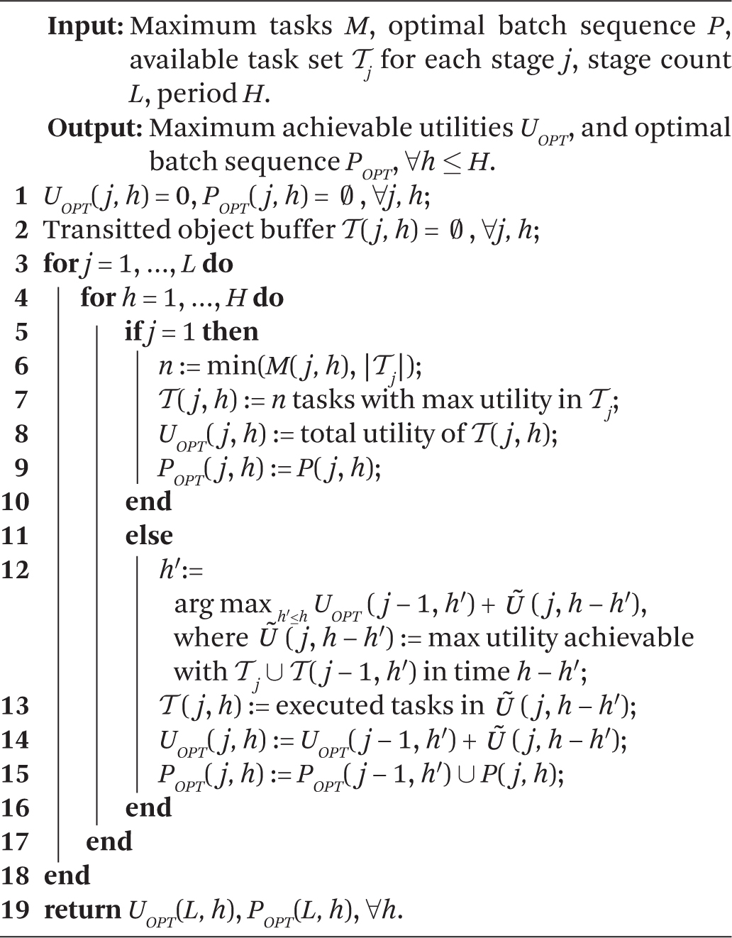
Step 2: We solve this problem by two-dimensional dynamic programming, considering the considered network stages and the time, respectively. The recursive (induction) step takes the output of Step 1 as input to calculate the optimal utility from assigning some fraction of Tk to the first j − 1 stage and the remainder to stage j, and computes the best possible sum of the two, for each Tk. Once all stages are considered, the result is the optimal utility, , from running tasks of input size k for a period Tk. The details are explained in Algorithm 2.
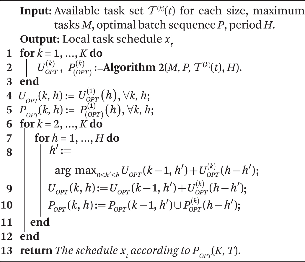
Step 3: Similar to Step 2, we perform a standard dynamic programming procedure to decide the optimal time partitioning among tasks processing different input sizes. The details of this procedure, along with the integrated local dynamic programming scheduling algorithm are presented in Algorithm 3.
The optimality of Algorithm 3 follows from the optimality of dynamic programming. Hence, the overall competitive ratio is 3 for single-stage task scheduling and min{L+2, 2B+1} for multi-stage task scheduling, according to Corollary 1 and Theorem 1, respectively. However, this algorithm may have a high computational overhead since Algorithms 2 and 3 which need to be executed each scheduling period, are O(KLH3). Next, we present a simpler local greedy algorithm, which has better time efficiency.
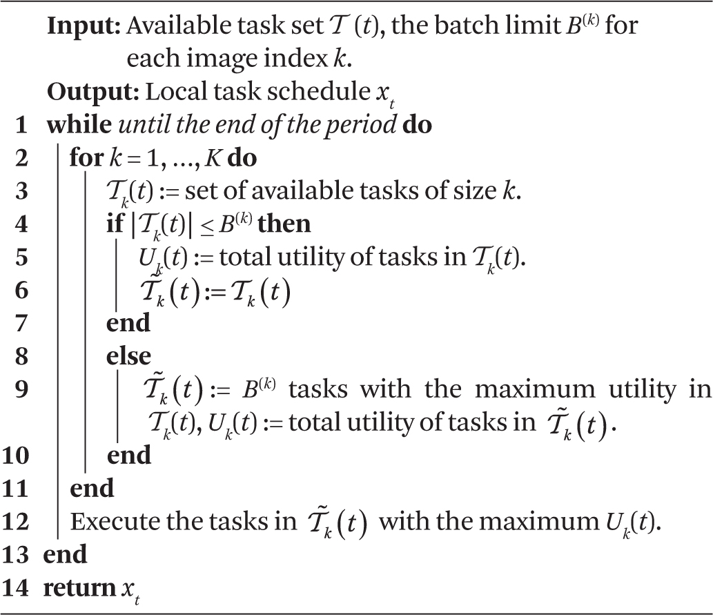
Local Greedy scheduling. The greedy online scheduling algorithm solves the local BASIC scheduling problem following a simple greedy selection rule: Execute the (eligible) batch with the maximum utility next. The pseudo-code of the greedy scheduling algorithm is shown in Algorithm 4. The greedy scheduling algorithm is simple to implement and has a very low computational overhead. We show that it achieves a comparable performance to the optimal algorithm in practice.
4. Evaluation
In this section, we verify the effectiveness and efficiency of our proposed scheduling framework by comparing it with several state-of-the-art baselines on a large-scale self-driving dataset, Waymo Open Dataset.
4.1. Experimental setup
Hardware platform. All experiments are conducted on an NVIDIA Jetson AGX Xavier SoC, which is specifically designed for automotive platforms. It’s equipped with an 8-core Carmel Arm v8.2 64-bit CPU, a 512-core Volta GPU, and 32GB memory. Its mode is set as MAXN with maximum CPU/GPU/memory frequency budget, and all CPU cores are online.
Dataset. Our experiment is performed on the Waymo Open Dataset,19 which is a large-scale autonomous driving dataset collected by Waymo self-driving cars in diverse geographies and conditions. It includes driving video segments of the 20s each, collected by LiDARs and cameras at 10Hz. Only the front camera data is used in our experiment.
Neural network training. We use ResNet proposed by He et al.10 for object classification. The network is trained on a general-purpose object detection dataset, COCO.13 It contains 80 object classes that cover Waymo classes.
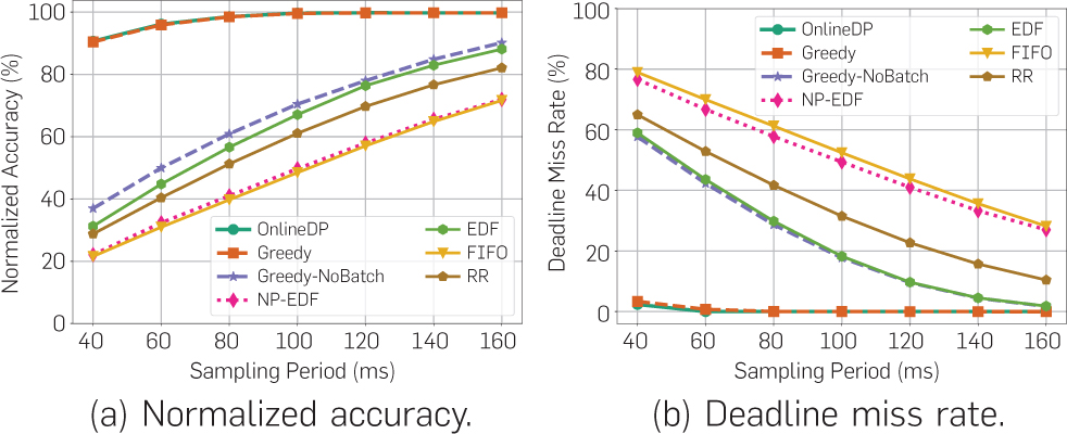
Scheduling load and evaluation metrics. We extract the distance between objects and the autonomous vehicle (AV) from the projected LiDAR point cloud. The deadlines of object classification tasks are set as the time to collision (TTC) with the AV. To simulate different loads for the scheduling algorithms, we manually change the sampling period (i.e., frame rate) from 40ms to 160ms. We consider a task to miss its deadline if the scheduler fails to run the mandatory part of the task by the deadline. In the following evaluation, we present both the normalized accuracy and deadline miss rate for different algorithms. The normalized accuracy is defined as the ratio between achieved accuracy and the maximum accuracy when all neural network stages are finished for every object.
4.2. Compared scheduling algorithms
The following scheduling algorithms are compared.
OnlineDP: the online scheduling algorithm we proposed in Section 3. The local scheduling is conducted by the hierarchical dynamic programming algorithm.
Greedy: the online scheduling algorithm we proposed, with the local scheduling conducted by the greedy batching algorithm.
Greedy-NoBatch: It always executes the object with maximal marginal utility without batching.
EDF: It always chooses the task stage with the earliest deadline (without considering task utility).
Non-Preemptive EDF (NP-EDF): This algorithm does not allow preemption. It is included to understand the impact of allowing preemption on stage boundaries compared to not allowing it.
FIFO: It runs the task with the earliest arrival time first. All stages are performed as long as the deadline is not violated.
RR: Round-robin scheduling algorithm. Runs one stage of each task in a round-robin fashion.
4.3. Slicing and batching
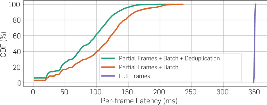
We compare the inference time for full frames and batched partial frames with/out deduplication. In full-frame processing, we directly run the neural network on image-captured full images, whose size is 1920 × 1280. In batched partial frames, we do the slicing into bounding boxes within one frame first, then perform the deduplication (if applicable), and finally, batch execution of objects with the same size. Each frame is evaluated independently. No imprecise computation is considered. Our results show that the average latency for full frames is 350ms, while the average latency for (the sum of) batched partial frames is 105ms without deduplication, and 83ms with deduplication. Besides, the cumulative distributions of frame latencies for the three methods are shown in Figure 4. Data slicing, batching, and deduplication steps, although induce extra processing delays, can effectively reduce the end-to-end latency. However, neither approach is fast enough compared to 100ms sampling period, so that the imprecise computation model and prioritization are needed.
4.4. Scheduling policy comparisons
Next, we evaluate the scheduling algorithms in terms of achieved classification accuracy and deadline miss rate. The scheduling results are presented in Figure 5. The two proposed algorithms, OnlineDP and Greedy, clearly outperform all the baselines with a large margin in all metrics. The improvement comes for two reasons: First, the integration of the imprecise computation model into neural networks makes the scheduler more flexible. It makes the neural network partially preemptive at the stage level, and gives the scheduler an extra degree of freedom (namely, deciding how much of each task to execute). Second, the involvement of batching simultaneously improves the model performance and alleviates deadline misses. The batching mechanism enables the GPU to be utilized at its highest parallel capacity. The deadline miss rates of both OnlineDP and Greedy are pretty close to 0 under any task load. We find Greedy shows similar performance as OnlineDP, though they possess different theoretical results. One practical reason is that the utility prediction function can not perfectly predict the utility for all future stages, where the OnlineDP scheduling can be negatively impacted.
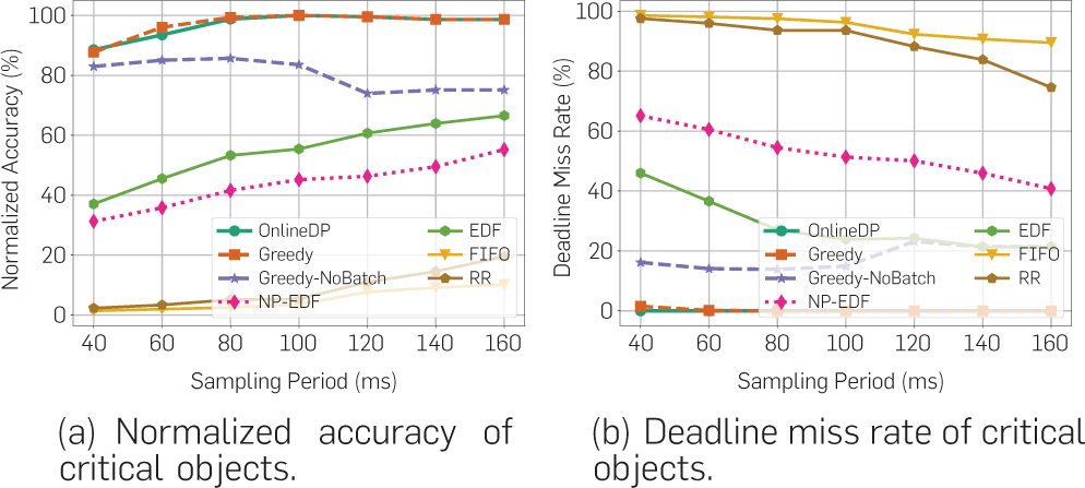
To evaluate scheduling performance in driving scenarios involving the aforementioned important subcases, we compare the metrics of different algorithms for the subset of “critical objects.” Critical objects are defined as objects whose time-to-collision (and hence processing deadline) fall within 1s from when they first appear in the scene. Results are shown in Figure 6. We notice that the accuracy and deadline miss rates of FIFO and RR are much worse in this case (because severe priority inversion occurs in these two algorithms). The deadline-driven algorithms (NP-EDF and EDF) can effectively resolve this issue because objects with earlier deadlines are always executed first. However, their general performance is limited for a lack of utility optimization. The utility-based scheduling algorithms (Greedy, Greedy-NoBatch, and OnlineDP) are also effective in removing priority inversion, while at the same time achieving better confidence in results. These algorithms multiply a weight factor a > 1 to increase the utility of handling critical objects so that they are preferred by the algorithm over non-critical ones.
5. Conclusion
We presented a novel perception pipeline architecture and scheduling algorithm that resolve algorithmic priority inversion in mission-critical machine inference pipelines, prevalent in conventional FIFO-based AI workflows. To mitigate the impact of priority inversion, the proposed online scheduling architecture rests on two key ideas: (1) Prioritize parts of the incoming sensor data over others to enable a more timely response to more critical stimuli, and (2) Explore the maximum parallel capacity of the GPU by a novel task batching algorithm that improves both response speed and quality. An extensive evaluation, performed on a real-world driving dataset, validates the effectiveness of our framework.
Acknowledgments
Research reported in this paper was sponsored in part by the Army Research Laboratory under Cooperative Agreement W911NF-17-20196, NSF CNS 18-15891, NSF CNS 18-15959, NSF CNS 19-32529, NSF CNS 20-38817, Navy N00014-17-1-2783, and the Boeing Company.






Join the Discussion (0)
Become a Member or Sign In to Post a Comment