
Thanks to advances in sensing, networking, and data management, our society is producing digital information at an astonishing rate. According to one estimate, in 2010 alone we will generate 1,200 exabytes—60 million times the content of the Library of Congress. Within this deluge of data lies a wealth of valuable information on how we conduct our businesses, governments, and personal lives. To put the information to good use, we must find ways to explore, relate, and communicate the data meaningfully.
The goal of visualization is to aid our understanding of data by leveraging the human visual system’s highly tuned ability to see patterns, spot trends, and identify outliers. Well-designed visual representations can replace cognitive calculations with simple perceptual inferences and improve comprehension, memory, and decision making. By making data more accessible and appealing, visual representations may also help engage more diverse audiences in exploration and analysis. The challenge is to create effective and engaging visualizations that are appropriate to the data.
Creating a visualization requires a number of nuanced judgments. One must determine which questions to ask, identify the appropriate data, and select effective visual encodings to map data values to graphical features such as position, size, shape, and color. The challenge is that for any given data set the number of visual encodings—and thus the space of possible visualization designs—is extremely large. To guide this process, computer scientists, psychologists, and statisticians have studied how well different encodings facilitate the comprehension of data types such as numbers, categories, and networks. For example, graphical perception experiments find that spatial position (as in a scatter plot or bar chart) leads to the most accurate decoding of numerical data and is generally preferable to visual variables such as angle, one-dimensional length, two-dimensional area, three-dimensional volume, and color saturation. Thus, it should be no surprise that the most common data graphics, including bar charts, line charts, and scatter plots, use position encodings. Our understanding of graphical perception remains incomplete, however, and must appropriately be balanced with interaction design and aesthetics.
This article provides a brief tour through the “visualization zoo,” showcasing techniques for visualizing and interacting with diverse data sets. In many situations, simple data graphics will not only suffice, they may also be preferable. Here we focus on a few of the more sophisticated and unusual techniques that deal with complex data sets. After all, you don’t go to the zoo to see chihuahuas and raccoons; you go to admire the majestic polar bear, the graceful zebra, and the terrifying Sumatran tiger. Analogously, we cover some of the more exotic (but practically useful) forms of visual data representation, starting with one of the most common, time-series data; continuing on to statistical data and maps; and then completing the tour with hierarchies and networks. Along the way, bear in mind that all visualizations share a common “DNA”—a set of mappings between data properties and visual attributes such as position, size, shape, and color—and that customized species of visualization might always be constructed by varying these encodings.
Each visualization shown here is accompanied by an online interactive example that can be viewed at the URL displayed beneath it. The live examples were created using Protovis, an open source language for Web-based data visualization. To learn more about how a visualization was made (or to copy and paste it for your own use), see the online version of this article available on the ACM Queue site at http://queue.acm.org/detail.cfm?id=1780401/. All example source code is released into the public domain and has no restrictions on reuse or modification. Note, however, that these examples will work only on a modern, standards-compliant browser supporting scalable vector graphics (SVG). Supported browsers include recent versions of Firefox, Safari, Chrome, and Opera. Unfortunately, Internet Explorer 8 and earlier versions do not support SVG and so cannot be used to view the interactive examples.
Time-Series Data
Sets of values changing over time—or, time-series data—is one of the most common forms of recorded data. Time-varying phenomena are central to many domains such as finance (stock prices, exchange rates), science (temperatures, pollution levels, electric potentials), and public policy (crime rates). One often needs to compare a large number of time series simultaneously and can choose from a number of visualizations to do so.
Index Charts. With some forms of time-series data, raw values are less important than relative changes. Consider investors who are more interested in a stock’s growth rate than its specific price. Multiple stocks may have dramatically different baseline prices but may be meaningfully compared when normalized. An index chart is an interactive line chart that shows percentage changes for a collection of time-series data based on a selected index point. For example, the image in Figure 1a shows the percentage change of selected stock prices if purchased in January 2005: one can see the rocky rise enjoyed by those who invested in Amazon, Apple, or Google at that time.
Stacked Graphs. Other forms of time-series data may be better seen in aggregate. By stacking area charts on top of each other, we arrive at a visual summation of time-series values—a stacked graph. This type of graph (sometimes called a stream graph) depicts aggregate patterns and often supports drill-down into a subset of individual series. The chart in Figure 1b shows the number of unemployed workers in the U.S. over the past decade, subdivided by industry. While such charts have proven popular in recent years, they do have some notable limitations. A stacked graph does not support negative numbers and is meaningless for data that should not be summed (temperatures, for example). Moreover, stacking may make it difficult to accurately interpret trends that lie atop other curves. Interactive search and filtering is often used to compensate for this problem.
Small Multiples. In lieu of stacking, multiple time series can be plotted within the same axes, as in the index chart. Placing multiple series in the same space may produce overlapping curves that reduce legibility, however. An alternative approach is to use small multiples: showing each series in its own chart. In Figure 1c we again see the number of unemployed workers, but normalized within each industry category. We can now more accurately see both overall trends and seasonal patterns in each sector. While we are considering time-series data, note that small multiples can be constructed for just about any type of visualization: bar charts, pie charts, maps, among others. This often produces a more effective visualization than trying to coerce all the data into a single plot.
Horizon Graphs. What happens when you want to compare even more time series at once? The horizon graph is a technique for increasing the data density of a time-series view while preserving resolution. Consider the five graphs shown in Figure 1d. The first one is a standard area chart, with positive values colored blue and negative values colored red. The second graph “mirrors” negative values into the same region as positive values, doubling the data density of the area chart. The third chart—a horizon graph—doubles the data density yet again by dividing the graph into bands and layering them to create a nested form. The result is a chart that preserves data resolution but uses only a quarter of the space. Although the horizon graph takes some time to learn, it has been found to be more effective than the standard plot when the chart sizes get quite small.
Statistical Distributions
Other visualizations have been designed to reveal how a set of numbers is distributed and thus help an analyst better understand the statistical properties of the data. Analysts often want to fit their data to statistical models, either to test hypotheses or predict future values, but an improper choice of model can lead to faulty predictions. Thus, one important use of visualizations is exploratory data analysis: gaining insight into how data is distributed to inform data transformation and modeling decisions. Common techniques include the histogram, which shows the prevalence of values grouped into bins, and the box-and-whisker plot, which can convey statistical features such as the mean, median, quartile boundaries, or extreme outliers. In addition, a number of other techniques exist for assessing a distribution and examining interactions between multiple dimensions.
Stem-and-Leaf Plots. For assessing a collection of numbers, one alternative to the histogram is the stem-and-leaf plot. It typically bins numbers according to the first significant digit, and then stacks the values within each bin by the second significant digit. This minimalistic representation uses the data itself to paint a frequency distribution, replacing the “information-empty” bars of a traditional histogram bar chart and allowing one to assess both the overall distribution and the contents of each bin. In Figure 2a, the stem-and-leaf plot shows the distribution of completion rates of workers completing crowd-sourced tasks on Amazon’s Mechanical Turk. Note the multiple clusters: one group clusters around high levels of completion (99%100%); at the other extreme is a cluster of Turkers who complete only a few tasks (~10%) in a group.
Q-Q Plots. Though the histogram and the stem-and-leaf plot are common tools for assessing a frequency distribution, the Q-Q (quantile-quantile) plot is a more powerful tool. The Q-Q plot compares two probability distributions by graphing their quantiles against each other. If the two are similar, the plotted values will lie roughly along the central diagonal. If the two are linearly related, values will again lie along a line, though with varying slope and intercept.
Figure 2b shows the same Mechanical Turk participation data compared with three statistical distributions. Note how the data forms three distinct components when compared with uniform and normal (Gaussian) distributions: this suggests that a statistical model with three components might be more appropriate, and indeed we see in the final plot that a fitted mixture of three normal distributions provides a better fit. Though powerful, the Q-Q plot has one obvious limitation in that its effective use requires that viewers possess some statistical knowledge.
SPLOM (Scatter Plot Matrix). Other visualization techniques attempt to represent the relationships among multiple variables. Multivariate data occurs frequently and is notoriously hard to represent, in part because of the difficulty of mentally picturing data in more than three dimensions. One technique to overcome this problem is to use small multiples of scatter plots showing a set of pairwise relations among variables, thus creating the SPLOM (scatter plot matrix). A SPLOM enables visual inspection of correlations between any pair of variables.
In Figure 2c a scatter plot matrix is used to visualize the attributes of a database of automobiles, showing the relationships among horsepower, weight, acceleration, and displacement. Additionally, interaction techniques such as brushing-and-linking—in which a selection of points on one graph highlights the same points on all the other graphs—can be used to explore patterns within the data.
Parallel Coordinates. As shown in Figure 2d, parallel coordinates (||-coord) take a different approach to visualizing multivariate data. Instead of graphing every pair of variables in two dimensions, we repeatedly plot the data on parallel axes and then connect the corresponding points with lines. Each poly-line represents a single row in the database, and line crossings between dimensions often indicate inverse correlation. Reordering dimensions can aid pattern-finding, as can interactive querying to filter along one or more dimensions. Another advantage of parallel coordinates is that they are relatively compact, so many variables can be shown simultaneously.
Maps
Although a map may seem a natural way to visualize geographical data, it has a long and rich history of design. Many maps are based upon a cartographic projection: a mathematical function that maps the 3D geometry of the Earth to a 2D image. Other maps knowingly distort or abstract geographic features to tell a richer story or highlight specific data.
Flow Maps. By placing stroked lines on top of a geographic map, a flow map can depict the movement of a quantity in space and (implicitly) in time. Flow lines typically encode a large amount of multivariate information: path points, direction, line thickness, and color can all be used to present dimensions of information to the viewer. Figure 3a is a modern interpretation of Charles Minard’s depiction of Napoleon’s ill-fated march on Moscow. Many of the greatest flow maps also involve subtle uses of distortion, as geography is bended to accommodate or highlight flows.
Choropleth Maps. Data is often collected and aggregated by geographical areas such as states. A standard approach to communicating this data is to use a color encoding of the geographic area, resulting in a choropleth map. Figure 3b uses a color encoding to communicate the prevalence of obesity in each state in the U.S. Though this is a widely used visualization technique, it requires some care. One common error is to encode raw data values (such as population) rather than using normalized values to produce a density map. Another issue is that one’s perception of the shaded value can also be affected by the underlying area of the geographic region.
Graduated Symbol Maps. An alternative to the choropleth map, the graduated symbol map places symbols over an underlying map. This approach avoids confounding geographic area with data values and allows for more dimensions to be visualized (for example, symbol size, shape, and color). In addition to simple shapes such as circles, graduated symbol maps may use more complicated glyphs such as pie charts. In Figure 3c, total circle size represents a state’s population, and each slice indicates the proportion of people with a specific BMI rating.
Cartograms. A cartogram distorts the shape of geographic regions so that the area directly encodes a data variable. A common example is to redraw every country in the world sizing it proportionally to population or gross domestic product. Many types of cartograms have been created; in Figure 3d we use the Dorling cartogram, which represents each geographic region with a sized circle, placed so as to resemble the true geographic configuration. In this example, circular area encodes the total number of obese people per state, and color encodes the percentage of the total population that is obese.
Hierarchies
While some data is simply a flat collection of numbers, most can be organized into natural hierarchies. Consider: spatial entities, such as counties, states, and countries; command structures for businesses and governments; software packages and phylogenetic trees. Even for data with no apparent hierarchy, statistical methods (for example, k-means clustering) may be applied to organize data empirically. Special visualization techniques exist to leverage hierarchical structure, allowing rapid multiscale inferences: micro-observations of individual elements and macro-observations of large groups.
Node-link diagrams. The word tree is used interchangeably with hierarchy, as the fractal branches of an oak might mirror the nesting of data. If we take a two-dimensional blueprint of a tree, we have a popular choice for visualizing hierarchies: a node-link diagram. Many different tree-layout algorithms have been designed; the Reingold-Tilford algorithm, used in Figure 4a on a package hierarchy of software classes, produces a tidy result with minimal wasted space.
An alternative visualization scheme is the dendrogram (or cluster) algorithm, which places leaf nodes of the tree at the same level. Thus, in the diagram in Figure 4b, the classes (orange leaf nodes) are on the diameter of the circle, with the packages (blue internal nodes) inside. Using polar rather than Cartesian coordinates has a pleasing aesthetic, while using space more efficiently.
We would be remiss to overlook the indented tree, used ubiquitously by operating systems to represent file directories, among other applications (see Figure 4c). Although the indented tree requires excessive vertical space and does not facilitate multiscale inferences, it does allow efficient interactive exploration of the tree to find a specific node. In addition, it allows rapid scanning of node labels, and multivariate data such as file size can be displayed adjacent to the hierarchy.
Adjacency Diagrams. The adjacency diagram is a space-filling variant of the node-link diagram; rather than drawing a link between parent and child in the hierarchy, nodes are drawn as solid areas (either arcs or bars), and their placement relative to adjacent nodes reveals their position in the hierarchy. The icicle layout in Figure 4d is similar to the first node-link diagram in that the root node appears at the top, with child nodes underneath. Because the nodes are now space-filling, however, we can use a length encoding for the size of software classes and packages. This reveals an additional dimension that would be difficult to show in a node-link diagram.
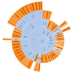
The sunburst layout, shown in Figure 4e, is equivalent to the icicle layout, but in polar coordinates. Both are implemented using a partition layout, which can also generate a node-link diagram. Similarly, the previous cluster layout can be used to generate a space-filling adjacency diagram in either Cartesian or polar coordinates.
Enclosure Diagrams. The enclosure diagram is also space filling, using containment rather than adjacency to represent the hierarchy. Introduced by Ben Shneiderman in 1991, a treemap recursively subdivides area into rectangles. As with adjacency diagrams, the size of any node in the tree is quickly revealed. The example shown in Figure 4f uses padding (in blue) to emphasize enclosure; an alternative saturation encoding is sometimes used. Squarified treemaps use approximately square rectangles, which offer better readability and size estimation than a naive “slice-and-dice” subdivision. Fancier algorithms such as Voronoi and jigsaw treemaps also exist but are less common.
By packing circles instead of subdividing rectangles, we can produce a different sort of enclosure diagram that has an almost organic appearance. Although it does not use space as efficiently as a treemap, the “wasted space” of the circle-packing layout, shown in Figure 4g, effectively reveals the hierarchy. At the same time, node sizes can be rapidly compared using area judgments.
Networks
In addition to organization, one aspect of data that we may wish to explore through visualization is relationship. For example, given a social network, who is friends with whom? Who are the central players? What cliques exist? Who, if anyone, serves as a bridge between disparate groups? Abstractly, a hierarchy is a specialized form of network: each node has exactly one link to its parent, while the root node has no links. Thus node-link diagrams are also used to visualize networks, but the loss of hierarchy means a different algorithm is required to position nodes.
Mathematicians use the formal term graph to describe a network. A central challenge in graph visualization is computing an effective layout. Layout techniques typically seek to position closely related nodes (in terms of graph distance, such as the number of links between nodes, or other metrics) close in the drawing; critically, unrelated nodes must also be placed far enough apart to differentiate relationships. Some techniques may seek to optimize other visual features—for example, by minimizing the number of edge crossings.
Force-directed Layouts. A common and intuitive approach to network layout is to model the graph as a physical system: nodes are charged particles that repel each other, and links are dampened springs that pull related nodes together. A physical simulation of these forces then determines the node positions; approximation techniques that avoid computing all pairwise forces enable the layout of large numbers of nodes. In addition, interactivity allows the user to direct the layout and jiggle nodes to disambiguate links. Such a force-directed layout is a good starting point for understanding the structure of a general undirected graph. In Figure 5a we use a force-directed layout to view the network of character co-occurrence in the chapters of Victor Hugo’s classic novel, Les Misérables. Node colors depict cluster memberships computed by a community-detection algorithm.
Arc Diagrams. An arc diagram, shown in Figure 5b, uses a one-dimensional layout of nodes, with circular arcs to represent links. Though an arc diagram may not convey the overall structure of the graph as effectively as a two-dimensional layout, with a good ordering of nodes it is easy to identify cliques and bridges. Further, as with the indented-tree layout, multivariate data can easily be displayed alongside nodes. The problem of sorting the nodes in a manner that reveals underlying cluster structure is formally called seriation and has diverse applications in visualization, statistics, and even archaeology.
Matrix Views. Mathematicians and computer scientists often think of a graph in terms of its adjacency matrix: each value in row i and column j in the matrix corresponds to the link from node i to node j. Given this representation, an obvious visualization then is: just show the matrix! Using color or saturation instead of text allows values associated with the links to be perceived more rapidly.
All visualizations share a common “DNA”—a set of mappings between data properties and visual attributes such as position, size, shape, and color—and customized species of visualization might always be constructed by varying these encodings.
The seriation problem applies just as much to the matrix view, shown in Figure 5c, as to the arc diagram, so the order of rows and columns is important: here we use the groupings generated by a community-detection algorithm to order the display. While path-following is more difficult in a matrix view than in a node-link diagram, matrices have a number of compensating advantages. As networks get large and highly connected, node-link diagrams often devolve into giant hairballs of line crossings. In matrix views, however, line crossings are impossible, and with an effective sorting one quickly can spot clusters and bridges. Allowing interactive grouping and reordering of the matrix facilitates even deeper exploration of network structure.
Conclusion
We have arrived at the end of our tour and hope the reader has found the examples both intriguing and practical. Though we have visited a number of visual encoding and interaction techniques, many more species of visualization exist in the wild, and others await discovery. Emerging domains such as bioinformatics and text visualization are driving researchers and designers to continually formulate new and creative representations or find more powerful ways to apply the classics. In either case, the DNA underlying all visualizations remains the same: the principled mapping of data variables to visual features such as position, size, shape, and color.
As you leave the zoo and head back into the wild, try deconstructing the various visualizations crossing your path. Perhaps you can design a more effective display?
Few, S.
Now I See It: Simple Visualization Techniques for Quantitative Analysis. Analytics Press, 2009.
Tufte, E.
The Visual Display of Quantitative Information. Graphics Press, 1983.
Tufte, E.
Envisioning Information. Graphics Press, 1990.
Ware, C.
Visual Thinking for Design. Morgan Kaufmann, 2008.
Wilkinson, L.
The Grammar of Graphics. Springer, 1999.
 Visualization Development Tools
Prefuse: Java API for information visualization.
Prefuse Flare: ActionScript 3 library for data visualization in the Adobe Flash Player.
Processing: Popular language and IDE for graphics and interaction.
Protovis: JavaScript tool for Web-based visualization.
The Visualization Toolkit: Library for 3D and scientific visualization.
![]() Related articles
Related articles
on queue.acm.org
A Conversation with Jeff Heer, Martin Wattenberg, and Fernanda Viégas
http://queue.acm.org/detail.cfm?id=1744741
Unifying Biological Image Formats with HDF5
Matthew T. Dougherty, Michael J. Folk, Erez Zadok, Herbert J. Bernstein, Frances C. Bernstein, Kevin W. Eliceiri, Werner Benger, Christoph Best
http://queue.acm.org/detail.cfm?id=1628215
Figures
 Figure 1a. Time-Series Data: Index chart of selected technology stocks, 20002010.
 Figure 1b. Time-Series Data: Stacked graph of unemployed U.S. workers by industry, 20002010.
 Figure 1c. Time-Series Data: Small multiples of unemployed U.S. workers, normalized by industry, 20002010.
 Figure 1d. Time-Series Data: Horizon graphs of U.S. unemployment rate, 20002010.
 Figure 2a. Statistical Distributions: Stem-and-leaf plot of Mechanical Turk participation rates.
 Figure 2b. Statistical Distributions: Q-Q plots of Mechanical Turk participation rates.
 Figure 2c. Statistical Distributions: Scatter plot matrix of automobile data.
 Figure 2d. Statistical Distributions: Parallel coordinates of automobile data.
 Figure 3a. Maps: Flow map of Napoleon’s March on Moscow, based on the work of Charles Minard.
 Figure 3b. Maps: Choropleth map of obesity in the U.S., 2008.
 Figure 3c. Maps: Graduated symbol map of obesity in the U.S., 2008.
 Figure 3d. Maps: Dorling cartogram of obesity in the U.S., 2008.
 Figure 4a. Hierarchies: Radial node-link diagram of the Flare package hierarchy.
 Figure 4b. Hierarchies: Cartesian node-link diagram of the Flare package hierarchy.
 Figure 4c. Hierarchies: Indented tree layout of the Flare package hierarchy.
 Figure 4d. Hierarchies: Icicle tree layout of the Flare package hierarchy.
 Figure 4e. Hierarchies: Sunburst (radial space-filling) layout of the Flare package hierarchy.
 Figure 4f. Hierarchies: Treemap layout of the Flare package hierarchy.
 Figure 4g. Hierarchies: Nested circles layout of the Flare package hierarchy.
 Figure 5a. Networks: Force-directed layout of Les Misérables character co-occurrences.
 Figure 5b. Networks: Arc diagram of Les Misérables character co-occurrences.
 Figure 5c. Networks: Matrix view of Les Misérables character co-occurrences.
From
![]()


Join the Discussion (0)
Become a Member or Sign In to Post a Comment