
Introduction
Deep learning has been highly successful in recent years and has led to dramatic improvements in multiple domains. Deep‐learning algorithms often generalize quite well in practice, namely, given access to labeled training data, they return neural networks that correctly label unobserved test data. However, despite much research our theoretical understanding of generalization in deep learning is still limited.
Neural networks used in practice often have far more learnable parameters than training examples. In such overparameterized settings, one might expect overfitting to occur, that is, the learned network might perform well on the training dataset and perform poorly on test data. Indeed, in overparameterized settings, there are many solutions that perform well on the training data, but most of them do not generalize well. Surprisingly, it seems that gradient‐based deep‐learning algorithmsa prefer the solutions that generalize well.40
Decades of research in learning theory suggest that in order to avoid overfitting one should use a model which is “not more expressive than necessary”. Namely, the model should be able to perform well on the training data, but should be as “simple” as possible. This idea goes back to the Occam’s Razor philosophical principle, which argues that we should prefer simple explanations over complicated ones. For example, in Figure 1 the data points are labeled according to a degree‐3 polynomial plus a small random noise, and we fit it with a degree‐3 polynomial (green) and with a degree‐8 polynomial (red). The degree‐8 polynomial achieves better accuracy on the training data, but it overfits and will not generalize well.
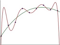
Figure 1:: Fitting training data with a degree‐3 polynomial (green) and degree‐8 polynomial (red). The latter achieves better accuracy on the training data but it overfits.
Simplicity in neural networks may stem from having a small number of parameters (which is often not the case in modern deep learning), but may also be achieved by adding a regularization term during the training, which encourages networks that minimize a certain measure of complexity. For example, we may add a regularizer that penalizes models where the Euclidean norm of the parameters (viewed as a vector) is large. However, in practice neural networks seem to generalize well even when trained without such an explicit regularization,40 and hence the success of deep learning cannot be attributed to explicit regularization. Therefore, it is believed that gradient‐based algorithms induce an implicit bias (or implicit regularization)28 which prefers solutions that generalize well, and characterizing this bias has been a subject of extensive research.
In this review article, we discuss the implicit bias in training neural networks using gradient‐based methods. The literature on this subject has rapidly expanded in recent years, and we aim to provide a high‐level overview of some fundamental results. This article is not a comprehensive survey, and there are certainly important results which are not discussed here.
The Double‐Descent Phenomenon
An important implication of the implicit bias in deep learning is the double‐descent phenomenon, observed by Belkin et al.6 As we already discussed, conventional wisdom in machine learning suggests that the number of parameters in the neural network should not be too large in order to avoid overfitting (when training without explicit regularization). Also, it should not be too small, in which case the model is not expressive enough and hence it performs poorly even on the training data, a situation called underfitting. This classical thinking can be captured by the U‐shaped risk (i.e., error or loss) curve from Figure 2(A). Thus, as we increase the number of parameters, the training risk decreases, and the test risk initially decreases and then increases. Hence, there is a “sweet spot” where the test risk is minimized. This classical U‐shaped curve suggests that we should not use a model that perfectly fits the training data.
The double‐descent phenomenon. Dashed lines denote the training risk and solid lines denote the test risk.
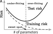
(A): The classical U‐shaped curve.
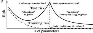
(B): The double‐descent curve, which extends the U‐shaped curve with a second descent. Beyond the “interpolation threshold” the model fits the training data perfectly, but the test risk decreases. The figure is from.6
However, it turns out that the U‐shaped curve only provides a partial picture. If we continue to increase the number of parameters in the model after the training set is already perfectly labeled, then there might be a second descent in the test risk (hence the name “double descent”). As can be seen in Figure 2(B), by increasing the number of parameters beyond what is required to perfectly fit the training set, the generalization improves. Hence, in contrast to the classical approach which seeks a sweet spot, we may achieve generalization by using overparameterized neural networks. Modern deep learning indeed relies on using highly overparameterized networks.
The double‐descent phenomenon is believed to be a consequence of the implicit bias in deep‐learning algorithms. When using overparameterized models, gradient methods converge to networks that generalize well by implicitly minimizing a certain measure of the network’s complexity. As we will see next, characterizing this complexity measure in different settings is a challenging puzzle.
Implicit Bias in Classification
We start with the implicit bias in classification tasks, namely, where the labels are in {−1,1}. Neural networks are trained in practice using the gradient‐descent algorithm and its variants, such as stochastic gradient descent (SGD). In gradient descent, we start from some random initialization θ0 of the network’s parameters, and then in each iteration t≥1 we update θt=θt−1−η∇ℒ(θt−1), where η>0 is the step size and ℒ is some empirical loss that we wish to minimize. Here, we will focus on gradient flow, which is a continuous version of gradient descent. That is, we train the parameters θ of the considered neural network, such that for all time t≥0 we have dθ(t)dt=−∇ℒ(θ(t)), where ℒ is the empirical loss, and θ(0) is some random initialization.b We focus on the logistic loss function (a.k.a. binary cross entropy): For a training dataset {(𝐱i,yi)}i=1n⊆ℝd×{−1,1} and a neural network 𝒩θ:ℝd→ℝ parameterized by θ, the empirical loss is defined by ℒ(θ)=1n∑i=1nlog(1+e−yi·𝒩θ(𝐱i)). We note that gradient flow corresponds to gradient descent with an infinitesimally small step size, and many implicit‐bias results are shown for gradient flow since it is often easier to analyze.
Logistic regression
Logistic regression is perhaps the simplest classification setting where implicit bias of neural networks can be considered. It corresponds to a neural network with a single neuron that does not have an activation function. That is, the model here is a linear predictor 𝐱↦𝐰⊤𝐱, where 𝐰∈ℝd are the learned parameters.
We assume that the data is linearly separable, i.e., there exists some 𝐰^∈ℝd such that for all i∈{1,…,n} we have yi·𝐰^⊤𝐱i>0. Note that ℒ(𝐰) is strictly positive for all 𝐰, but it may tend to zero as ǁ𝐰ǁ2 tends to infinity. For example, for α∈ℝ and 𝐰=α𝐰^ (where 𝐰^ is the vector defined above) we have limα→∞ℒ(𝐰)=0. However, there might be infinitely many directions 𝐰^ that satisfy this condition. Interestingly, Soudry et al.33 showed that gradient flow converges in direction to the ℓ2 maximum‐margin predictor. That is, 𝐰~=limt→∞𝐰(t)∥𝐰(t)∥2 exists, and 𝐰~ points at the direction of the maximum‐margin predictor, defined by
argmin w ∈ ℝ d ∥ w ∥ 2 s .t . ∀ i ∈ { 1 , … , n } y i ⋅ w ⊤ x i ≥ 1.The above characterization of the implicit bias in logistic regression can be used to explain generalization. Consider the case where d>n, thus, the input dimension is larger than the size of the dataset, and hence there are infinitely many vectors 𝐰 with ∥𝐰∥2=1 such that for all i∈{1,…,n} we have yi·𝐰⊤𝐱i>0, i.e., there are infinitely many directions that correctly label the training data. Some of the directions which fit the training data generalize well, and others do not. The above result guarantees that gradient flow converges to the maximum‐margin direction. Consequently, we can explain generalization by using standard margin‐based generalization bounds (cf.32), which imply that predictors achieving large margin generalize well.
Linear networks
We turn to deep neural networks where the activation is the identity function. Such neural networks are called linear networks. These networks compute linear functions, but the network architectures induce significantly different dynamics of gradient flow compared to the case of linear predictors 𝐱↦𝐰⊤𝐱 that we already discussed. Hence, the implicit bias in linear networks has been extensively studied, as a first step towards understanding implicit bias in deep nonlinear networks. It turns out that understanding implicit bias in linear networks is highly non‐trivial, and its study reveals valuable insights.
A linear fully‐connected network 𝒩:ℝd→ℝ of depth k computes a function 𝒩(𝐱)=Wk…W1𝐱, where W1,…,Wk are weight matrices (where Wk is a row vector). The trainable parameters are a collection θ=[W1,…,Wk] of the weight matrices. By17,c if gradient flow converges to zero loss, namely, limt→∞ℒ(θ(t))=0, then the vector W1·…·Wk converges in direction to the ℓ2 maximum‐margin predictor. That is, although the dynamics of gradient flow in the case of a deep fully‐connected linear network is significantly different compared to the case of a linear predictor, in both cases gradient flow is biased towards the ℓ2 maximum‐margin predictor. We also note that by,16 the weight matrices W1,…,Wk−1 converge to matrices of rank 1. Thus, gradient flow on fully‐connected linear networks is also biased towards rank minimization of the weight matrices.
Once we consider linear networks which are not fully connected, gradient flow no longer maximizes the ℓ2 margin. For example, Gunasekar et al.13 showed that in linear diagonal networks (i.e., where the weight matrices W1,…,Wk−1 are diagonal) gradient flow encourages predictors that maximize the margin w.r.t. the ∥·∥2/k quasi‐norm. As a result, diagonal networks are biased towards sparse linear predictors. In linear convolutional networks they proved bias towards sparsity of the linear predictors in the frequency domain (see also39).
Homogeneous neural networks
Neural networks of practical interest have nonlinear activations and compute nonlinear predictors. The notion of margin maximization in nonlinear predictors is generally not well‐defined. Nevertheless, it has been established that for certain neural networks gradient flow maximizes the margin in parameter space. Thus, while in linear networks we considered margin maximization in predictor space (a.k.a. function space), here we consider margin maximization w.r.t. the network’s parameters.
Consider a neural network with parameters θ, denoted by 𝒩θ:ℝd→ℝ. We say that 𝒩θ is homogeneous if there exists L>0 such that for every α>0 and θ,𝐱 we have 𝒩α·θ(𝐱)=αL𝒩θ(𝐱). Here we think about θ as a vector obtained by concatenating all the parameters. That is, in homogeneous networks, scaling the parameters by any factor α>0 scales the predictions by αL. We note that a feedforward neural network with the ReLU activation (namely, z↦max{0,z}) is homogeneous if it does not contain skip‐connections (i.e., residual connections), and does not have bias terms, except maybe for the first hidden layer. Also, we note that a homogeneous network might include convolutional layers. In papers by Lyu and Li21 and by Ji and Telgarsky17,d it was shown that if gradient flow on homogeneous networks reaches a sufficiently small loss (at some time t0), then as t→∞ it converges to zero loss, the parameters converge in direction, i.e., θ~=limt→∞θ(t)∥θ(t)∥2 exists, and θ~ is biased towards margin maximization in the following sense. Consider the following margin maximization problem in parameter space:
min θ 1 2 ∥ θ ∥ 2 2 s.t. ∀ i ∈ { 1 , … , n } y i 𝒩 θ ( 𝐱 i ) ≥ 1 .Then, θ~ points at the direction of a first‐order stationary point of the above optimization problem, which is also called Karush–Kuhn–Tucker point, or KKT point for short. The KKT approach allows inequality constraints and is a generalization of the method of Lagrange multipliers, which allows only equality constraints.
A KKT point satisfies several conditions (called KKT conditions), and it was proved in21 that in the case of homogeneous neural networks these conditions are necessary for optimality. However, they are not sufficient even for local optimality (cf.35). Thus, a KKT point may not be an actual optimum of the maximum‐margin problem. It is analogous to showing that some unconstrained optimization problem converges to a point where the gradient is zero, without proving that it is a global/local minimum. Intuitively, convergence to a KKT point of the maximum‐margin problem implies a certain bias towards margin maximization in parameter space, although it does not guarantee convergence to a maximum‐margin solution.
As we already discussed, in linear classifiers and linear neural networks, margin maximization (in predictor space) can explain generalization using well‐known margin‐based generalization bounds. Can margin maximization in parameter space explain generalization in nonlinear neural networks? In recent years several works showed margin‐based generalization bounds for neural networks (e.g.,5,11). Hence, generalization in neural networks might be established by combining these results with results on the implicit bias towards margin maximization in parameter space. On the flip side, we note that it is still unclear how tight the known margin‐based generalization bounds for neural networks are, and whether the sample complexity implied by such results (i.e., the required size of the training dataset) may be small enough to capture the situation in practice.
Several results on implicit bias were shown for some specific cases of nonlinear homogeneous networks. For example:8 showed bias towards margin maximization w.r.t. a certain function norm (known as the variation norm) in infinite‐width two‐layer homogeneous networks;22 proved margin maximization in two‐layer Leaky‐ReLU networks trained on linearly separable and symmetric data, and31 proved convergence to a linear classifier in two‐layer Leaky‐ReLU networks under different assumptions;30 showed bias towards minimizing the number of linear regions in univariate two‐layer ReLU networks.
Finally, the implicit bias in non‐homogeneous neural networks (such as ResNets) is currently not well‐understood.e Improving our knowledge of non‐homogeneous networks is an important challenge in the path towards understanding implicit bias in deep learning.
Extensions
For simplicity, we considered so far only gradient flow in binary classification. We note that many of the above results can also be extended to other gradient methods (such as gradient descent, steepest descent and SGD), and to multiclass classification with the cross‐entropy loss. The results can also be extended to various loss functions. Furthermore, we focused on an asymptotic analysis, i.e., where the time t tends to infinity, but the analysis can be extended to the case where gradient descent is trained for a finite number of iterations. We discuss all the above important extensions in the appendix. Additional aspects of the implicit bias, which apply both to classification and regression, are discussed in Sections 5 and 6.
Implicit Bias in Regression
We turn to consider the implicit bias of gradient methods in regression tasks, namely, where the labels are in ℝ. We focus on gradient flow and on the square‐loss function. Thus, we have dθ(t)dt=−∇ℒ(θ(t)), where the empirical loss ℒ(θ) is defined such that given a training dataset {(𝐱i,yi)}i=1n⊆ℝd×ℝ and a neural network 𝒩θ:ℝd→ℝ, we have ℒ(θ)=1n∑i=1n(𝒩θ(𝐱i)−yi)2. In an overparameterized setting, there might be many possible choices of θ such that ℒ(θ)=0, thus there are many global minima. Ideally, we want to find some implicit regularization function ℛ(θ) such that gradient flow prefers global minima which minimize ℛ. That is, if gradient flow converges to some θ* with ℒ(θ*)=0, then we have θ*∈argminθℛ(θ) s.t.ℒ(θ)=0.
Linear regression
We start with linear regression, which is perhaps the simplest regression setting where the implicit bias of neural networks can be considered. Here, the model is a linear predictor 𝐱↦𝐰⊤𝐱, where 𝐰∈ℝd are the learned parameters. In this case, it is not hard to show that gradient flow converges to the global minimum of ℒ(𝐰), which is closest to the initialization 𝐰(0) in ℓ2 distance.12,40 Thus, the implicit regularization function is ℛ𝐰(0)(𝐰)=∥𝐰−𝐰(0)∥2. Minimizing this ℓ2 norm allows us to explain generalization using standard norm‐based generalization bounds.32
We note that the results on linear regression can be extended to optimization methods other than gradient flow, such as gradient descent, SGD, and mirror descent.3,12,f
Linear networks
A linear neural network 𝒩θ:ℝd→ℝ has the identity activation function and computes a linear predictor 𝐱↦𝐰⊤𝐱, where 𝐰 is the vector obtained by multiplying the weight matrices in 𝒩θ. Hence, instead of seeking an implicit regularization function ℛ(θ) we may aim to find ℛ(𝐰). Similarly to our discussion in the context of classification, the network architectures in deep linear networks induce significantly different dynamics of gradient flow compared to the case of linear regression. Hence, the implicit bias in such networks has been studied as a first step towards understanding implicit bias in deep nonlinear networks.
Exact expressions for ℛ(𝐰) have been obtained for linear diagonal networks and linear fully‐connected networks.4,36,39 The expressions for ℛ(𝐰) are rather complicated, and depend on the initialization scale, i.e., the norm of 𝐰(0), and the initialization “shape”, namely, the relative magnitudes of different weights and layers in the network. Below we discuss a few special cases.
Recall that diagonal networks are neural networks where the weight matrices are diagonal. The regularization function ℛ has been obtained for a few variants of diagonal networks. In36 the authors considered networks of the form 𝐱↦(𝐮+∘𝐮+−𝐮−∘𝐮−)⊤𝐱, where 𝐮+,𝐮−∈ℝd and the operator ∘ denotes the Hadamard (entrywise) product. Thus, in this network, which can be viewed as a variant of a diagonal network, the weights in the two layers are shared. For an initialization 𝐮+(0)=𝐮−(0)=α·1, the scale α>0 of the initialization does not affect 𝐰(0)=𝐮+(0)∘𝐮+(0)−𝐮−(0)∘𝐮−(0)=0. However, the initialization scale does affect the implicit bias: if α→0 then ℛ(𝐰)=∥𝐰∥1 and if α→∞ (which corresponds to the so‐called kernel regime) then ℛ(𝐰)=∥𝐰∥2. Thus, the implicit bias transitions between the ℓ1 norm and the ℓ2 norm as we increase the initialization scale. A similar result holds also for deeper networks. In two‐layer “diagonal networks” with a similar structure, but where the weights are not shared,4 showed that the implicit bias is affected by both the initialization scale and “shape”. In39 the authors showed a transition between the ℓ1 and ℓ2 norms both in diagonal networks and in certain convolutional networks (in the frequency domain).
In two‐layer fully‐connected linear networks with infinitesimally small initialization, gradient flow minimizes the ℓ2 norm, namely, ℛ(𝐰)=∥𝐰∥2.4,39 This result was shown also for deep fully‐connected linear networks, under certain assumptions on the initialization.39
Some additional aspects of the implicit bias in linear networks are discussed in Sections 5 and 6.
Matrix factorization as a test‐bed for neural networks
Towards the goal of understanding implicit bias in neural networks, much effort was directed at the matrix factorization (and more specifically, matrix sensing) problem. In this problem, we are given a set of observations about an unknown matrix W*∈ℝd×d and we find a matrix W=W2W1 with W1,W2∈ℝd×d that is compatible with the given observations by running gradient flow. More precisely, consider the observations {(Xi,yi)}i=1n⊆ℝd×d×ℝ such that yi=〈W*,Xi〉, where in the inner product we view W* and Xi as vectors (namely, 〈W,X〉=tr(W⊤X)). Then, we find W=W2W1 using gradient flow on the objective ℒ(W1,W2)=1n∑i=1n(〈W2W1,Xi〉−yi)2. Since W1,W2∈ℝd×d then the rank of W is not limited by the parameterization. However, the parameterization has a crucial effect on the implicit bias. Assuming that there are many matrices W that are compatible with the observations, the implicit bias controls which matrix gradient flow finds. A notable special case of matrix sensing is matrix completion. Here, every observation has the form Xi=𝐞pi𝐞qi⊤, where {𝐞1,…,𝐞d} is the standard basis. Thus, each observation (Xi,yi) reveals a single entry from the matrix W*.
The matrix factorization problem is analogous to training a two‐layer linear network. Furthermore, we may consider deep matrix factorization where we have W=WkWk−1…W1, which is analogous to training a deep linear network. Therefore, this problem is considered a natural test‐bed to investigate implicit bias in neural networks, and has been studied extensively in recent years (e.g.,1,14,19,20,29).
Gunasekar et al.14 conjectured that in matrix factorization, the implicit bias of gradient flow starting from small initialization is given by the nuclear norm of W (a.k.a. the trace norm). That is, ℛ(W)=∥W∥*. They also proved this conjecture in the restricted case where the matrices {Xi}i=1n commute. The conjecture was further studied in a line of works (e.g.,1,19,29) providing positive and negative evidence, and was formally refuted by.20 In29 the authors showed that gradient flow in matrix completion might approach a global minimum at infinity rather than converging to a global minimum with a finite norm. This result suggests that the implicit bias in matrix factorization may not be expressible by any norm or quasi‐norm. They conjectured that the implicit bias can be explained by rank minimization rather than norm minimization. In,20 the authors provided theoretical and empirical evidence that gradient flow with infinitesimally small initialization in the matrix‐factorization problem is mathematically equivalent to a simple heuristic rank‐minimization algorithm called Greedy Low‐Rank Learning.
Overall, although an explicit expression for a function ℛ is not known in the case of matrix factorization, we can view the implicit bias as a heuristic for rank minimization. It is still unclear what the implications of these results are for more practical nonlinear neural networks.
Nonlinear networks
Once we consider nonlinear networks the situation is even less clear. For a single‐neuron network, namely, 𝐱↦σ(𝐰⊤𝐱), where σ:ℝ→ℝ is strictly monotonic, gradient flow converges to the closest global minimum in ℓ2 distance, similarly to the case of linear regression. Thus, we have ℛ𝐰(0)(𝐰)=∥𝐰−𝐰(0)∥2. However, if σ is the ReLU activation then the implicit bias is not expressible by any non‐trivial function of 𝐰. A bit more precisely, suppose that ℛ:ℝd→ℝ is such that if gradient flow starting from 𝐰(0)=0 converges to a zero‐loss solution 𝐰*, then 𝐰* is a zero‐loss solution that minimizes ℛ. Then, such a function ℛ must be constant in ℝd{0}. Hence, the approach of precisely specifying the implicit bias of gradient flow via a regularization function is not feasible in single‐neuron ReLU networks.34 It suggests that this approach may not be useful for understanding implicit bias in the general case of ReLU networks.
On the positive side, in single‐neuron ReLU networks the implicit bias can be expressed approximately, within a factor of 2, by the ℓ2 norm. Namely, let 𝐰* be a zero‐loss solution with a minimal ℓ2 norm, and assume that gradient flow converges to some zero‐loss solution 𝐰(∞), then ∥𝐰(∞)∥2≤2∥𝐰*∥2.34
For two‐layer Leaky‐ReLU networks with a single hidden neuron, an explicit expression for ℛ was obtained in.4 However, if we replace the Leaky‐ReLU activation with ReLU, then the implicit bias is not expressible by any non‐trivial function, similarly to the case of a single‐neuron ReLU network.34
Overall, our understanding of implicit bias in nonlinear networks with regression losses is very limited. While in classification we have a useful characterization of the implicit bias in nonlinear homogeneous models, here we do not understand even extremely simple models. Improving our understanding of this question is a major challenge for the upcoming years.
In what follows, we will discuss some additional aspects of the implicit bias, which apply both to regression and classification.
Dynamical Stability
In the previous sections, we mostly focused on implicit bias in gradient flow, and also discussed cases where the results on gradient flow can be extended to other gradient methods. However, when considering gradient descent or SGD with a finite step size (rather than infinitesimal), the discrete nature of the algorithms and the stochasticity induce additional implicit biases that do not exist in gradient flow. These biases are crucial for understanding the behavior of gradient methods in practice, as empirical results suggest that increasing the step size and decreasing the batch size may improve generalization (cf.15,18).
It is well known that gradient descent and SGD cannot stably converge to minima that are too sharp relative to the step size (see, e.g.,24,25,27,37). Namely, in a stable minimum, the maximal eigenvalue of the Hessian is at most 2/η, where η is the step size. As a result, when using an appropriate step size we can rule out stable convergence to certain (sharp) minima, and thus encourage convergence to flat minima, which are believed to generalize better.18,37 Similarly, small batch sizes in SGD also encourage flat minima.18,23,37,38
We note that a function might be represented with many different networks, i.e., there are many sets of parameters that correspond to the same function. However, it is possible that some of these representations are sharp (in parameter space) and others are flat (cf.10). As a result, understanding the implications in function space of the bias towards flat minima (in parameter space) is often a challenging question.
Implications of the implicit bias towards flat minima were studied in several works. For example,25 studied flat minima in univariate ReLU networks, and showed that SGD with large step size is biased towards functions whose second derivative (w.r.t. the input) has a bounded weighted ℓ1 norm, which encourages convergence to smooth functions;27 showed that gradient descent with large step size on a diagonal linear network with non‐centered data minimizes the ℓ1 norm of the corresponding linear predictor, even in settings where gradient descent with small step size minimizes the ℓ2 norm;23 studied minima stability in SGD, and showed that flat minima induce regularization of the function’s gradient (w.r.t. the input data), and more generally that SGD regularizes Sobolev seminorms of the function;24 studied flat minima in linear neural networks, and showed bias towards solutions where the magnitudes of the layers are balanced, as well as other properties of flat solutions. We note that all the above papers consider regression with the square loss.
An intriguing related phenomenon, observed by Cohen et al.,9 is the tendency of gradient descent to operate in a regime called the Edge of Stability (EoS). They showed empirically for several architectures and tasks, and for both the cross‐entropy and the square loss, that the behavior of gradient descent with step size η consists of two stages. First, the loss curvature grows until the sharpness touches the bound of 2/η. Then, gradient decent enters the EoS regime, where curvature hovers around this bound, and the train loss behaves non‐monotonically, yet consistently decreases over long timescales. This phenomenon is not well understood, as traditional convergence analyses of gradient descent do not apply when the sharpness is above 2/η. The study of the EoS regime may contribute to our understanding of the dynamics and implicit bias in gradient descent and SGD. It was investigated in several recent theoretical works. For example,2 showed that training with modified gradient descent or modified loss (for a large family of losses) provably enters the EoS regime, and that the loss decreases in a non‐monotone manner, and7 studied EoS in training a two‐layer single‐neuron ReLU network with the square loss.
Additional Implicit Biases and Further Implications
Additional aspects of the implicit bias were studied in the literature. These aspects include the effect of label noise on the implicit bias in SGD; transforming gradient descent and SGD into gradient flow on a modified loss; balancedness of weights’ magnitudes between different layers; implications of norm minimization in parameter space on the predictor in function space; as well as implicit bias in the NTK regime. We briefly discuss these aspects in the appendix.
Moreover, we discuss in the appendix further implications of the implicit bias other than generalization, namely, implications on adversarial robustness and on privacy.
Conclusion
Deep‐learning algorithms exhibit remarkable performance, but it is not well‐understood why they are able to generalize despite having much more parameters than training examples. Exploring generalization in deep learning is an intriguing puzzle with both theoretical and practical implications. It is believed that implicit bias is a main ingredient in the ability of deep‐learning algorithms to generalize, and hence it has been widely studied.
Our understanding of implicit bias improved dramatically in recent years, but is still far from satisfactory. We believe that further progress in the study of implicit bias will eventually shed light on the mystery of generalization in deep learning.
Gal Vardi, TTI-Chicago and Hebrew University, USA


Join the Discussion (0)
Become a Member or Sign In to Post a Comment