A Unifying Framework for Incompleteness, Inconsistency, and Uncertainty in Databases

Databases are often assumed to have definite content. The reality, though, is that the database at hand may be deficient due to missing, invalid, or uncertain information. As a simple illustration, the primary address of a person may be missing, or it may conflict with another primary address, or it may be improbable given the presence of nearby businesses. A common practice to address this challenge is to rectify the database by fixing the gaps, as done in data imputation, entity resolution, and data cleaning. The process of rectifying the database, however, may involve arbitrary choices due to computational limitations, such as errors in statistical or machine-learning models, or mere lack of information that even humans cannot cope with in full confidence. In turn, answers to queries over the deficient database may depend on the choices made to rectify it; thus, the answers to queries may vary from one choice to choice, even though both choices may be equally legitimate.

In the pursuit of principled solutions, there has been a continuous research effort to develop fundamental approaches for handling database deficiency with no (or with less) arbitrariness. The purpose of this review article is to highlight some of the ways in which the possible world semantics has been deployed as a principled approach to overcome database deficiency in different contexts. In this approach, we acknowledge that we need to rectify the deficiency: fill in missing information, delete wrong records (hereafter tuples or facts), correct erroneous values, and so on. Yet, since many rectifications may exist and since we do not know which is the correct one, we do not commit to a specific one. Instead, we view our deficient database as a representation of the results of all conceivable rectifications, each such rectification giving rise to a legitimate candidate of a valid database that we call a possible world.

Since the possible worlds differ from each other, a query may produce different collections of answers (which are also tuples) when applied to different possible worlds. Therefore, query answering requires the use of an aggregation method to combine the query results over the possible worlds. The intersection of all possible results is the prototypical example of such an aggregation method. In this context, the tuples in the intersection are called the “certain answers” because they are obtained in every possible world, regardless of what rectification has led to it. Intersection is the most studied aggregation method because of its intuitive meaning: it extracts the answers for which validity is not affected by the database anomaly. For example, if we have uncertainty regarding the apartment number of a person $x$, we can still be certain about $x$ living in Paris in the same apartment as $y$. Intersection is the main, but not the only, aggregation method discussed in this survey. The union is a different type of aggregation, where we are interested in the “possible answers,” that is, the answers that are obtained in at least one possible world. Probabilistic variants of the possible world semantics have also been studied in depth; here, each rectification has a probability (that can be determined from the database content), and then the aggregation is done by marginal inference: to each tuple, we associate the probability that it is an answer when the query is applied to a random possible world.

It is often the case that the original (deficient) database constitutes a compact representation of the set of possible worlds, and that this set is infeasible to materialize or store; for example, the number of possible worlds can be exponential in the size of the representation or even infinite. Consequently, finding the certain answers to queries poses a significant computational challenge because an efficient aggregation of the answers over all possible worlds has to be performed without actually accessing each possible world, but by directly processing the compact deficient database. Such processing might be attainable for some queries but unattainable for others, and in such cases we would like to distinguish between queries with tractable and intractable certain answers. The distinction is often achieved via dichotomy theorems that classify the complexity of the certain answers of every query in some large family of queries.

We will illustrate the possible-world semantics in four different settings. While not exhaustive, these four settings represent substantially different mechanisms for forming possible worlds. In the setting of data exchange, logical inference rules are used to form the possible worlds: we have a database under one schema that has to be transformed into a database under a different schema, and the possible worlds are the candidate solutions according to rule-based constraints specifying the relationship between the two schemas. In the setting of inconsistent databases, minimal intervention is used to form the possible worlds: we have a database that violates integrity constraints, and the possible worlds are the different ways to repair the inconsistent database. In the setting of probabilistic databases, we have a representation of a probability distribution over the collection of all databases. Here we focus on the most studied model, the tuple-independent databases: each record has a confidence value that is interpreted as a probability, and different records are probabilistically independent. Finally, in the setting of election databases, completions of partial orders are used to form possible worlds: we have ordinary databases that describe information about voters, candidates, and winners in elections, but only partial knowledge about voter preferences is known, thus there is uncertainty about who the winning candidates are. Note that the framework of election databases augments computational social choice with relational database context. In particular, it generalizes the necessary winners and the possible winners problems studied by researchers in computational social choice, because we can now ask for the certainty or possibility of properties of the winners (for example, their partisan affiliation or position on some issue) and not just their mere identity (for example, whether candidate $a$ or candidate $b$ is a winner).

In each setting considered here, we use the lens of computational complexity to highlight the algorithmic aspects of aggregating the answers to conjunctive queries, an extensively studied class of queries that form the core of most relational database queries.

An online appendix (available at https://dl.acm.org/doi/10.1145/3624717) contains additional discussion about topics not covered in this article and an expanded list of references.

Basic Notions

  SELECT B.id2
  FROM Country C, Borders B
  WHERE C.id = B.id1 and C.name = "France"

Possible worlds and certain answers.

The standard query evaluation problem involves a query $q$ and an instance $I$, and the problem is to compute the answer $q\left(I\right)$ of $q$ on $I$. We explore settings where query evaluation involves a query and a collection of databases, instead of a single database. These databases can be thought of as possible worlds on which a query can be evaluated. What is the semantics of a query posed on different worlds? Clearly, we need a notion that provides a method for aggregating the answers obtained on each possible world. The certain answers is the most extensively studied such notion, where intersection is used as the aggregation method.

Definition 2.1.

Let $q$ be a $k$-ary query and let $W$ be a collection of databases. The certain answers of $q$ on $W$ is the set$$\text{CERTAIN}(q,W)=\bigcap _{J\in W}q\left(J\right)=\{a:a\in q\left(J\right),\text{for}\text{every}J\text{in}W\}.$$

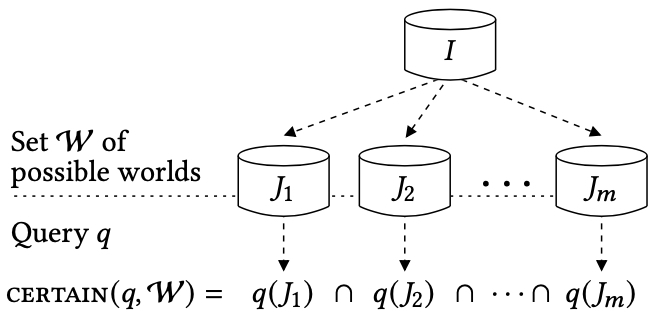
We will discuss the cost of computing the certain answers. On the face of their definition, computing the certain answers requires evaluating the query on each possible world. This may be a formidable task because the number of possible worlds can be very large or even infinite. In several different settings, however, the collection $W$ of the possible worlds admits a compact representation $ℛ$. This suggests a different approach: compute the certain answers of a query on $W$ by working with the compact representation $ℛ$, instead of examining each possible world in $W$.

We assume familiarity with basic notions in complexity theory, such as the complexity classes P, NP, coNP, and #P, and the meaning of hardness and completeness for complexity classes.¹⁸ We follow the convention of analyzing database problems in terms of their data complexity, which means that the input consists of the instance $I$ while everything else, such as the schema and the query, are fixed.³⁵ In particular, when we analyze computational problems associated with queries, each query gives rise to a separate computational problem, and this problem might be tractable for one query and intractable for another query.

Nulls and Data Exchange

In many settings, the possible worlds under consideration involve the use of null values that, intuitively, are placeholders for missing values. Database systems supported null values from the very beginning. Moreover, the pioneering work of Imielinski and Lipski²⁰ gave semantics to null values by means of possible worlds. Their framework introduced the concept of marked nulls, later called labeled nulls, that behave like variables: two occurrences of the same labeled null represent the same missing value, while distinct labeled nulls represent missing values that may be different or equal.

We will use the symbols $N_1,N_2,\dots$ to denote labeled nulls. An incomplete database $I$ is a collection of relations $R_1^I,\dots ,R_k^I$ such that each tuple $(a_1,\dots ,a_n)$ in each relation $R_i^I$ of $I$ consists of constants and labeled nulls, that is, each $a_j$ is a constant or a labeled null. Let $W\left(I\right)$ be the collection of all databases obtained from $I$ by replacing each labeled null by some constant. Therefore, the incomplete database $I$ is a compact representation of the possible worlds in $W\left(I\right)$. In this scenario, it is not hard to prove that the certain answers of a conjunctive query on $W\left(I\right)$ can be computed by evaluating the query directly on the compact representation $I$, where each labeled null in $I$ is treated as a distinct actual value (constant). More precisely, $\text{CERTAIN}(q,W\left(I\right))=q{\left(I\right)}_{\downarrow }$, where $q{\left(I\right)}_{\downarrow }$ is the set of of all null-free tuples of $q\left(I\right)$. For more details, Abiteboul et al.¹

In the SQL standard, nulls are not labeled, that is, there is a single null each occurrence of which should be viewed as a distinct labeled null. It should be noted that SQL queries do not adopt the certain-answer semantics, but rather the semantics of three-valued logic, where every comparison to a null value results in “unknown” rather than “true” or “false”. There has been a large body of work, such as Libkin’s,²⁸ in which the SQL semantics are compared and contrasted with the certain-answer semantics.

The preceding uses of nulls have been extensively studied, and we will not focus on these here. Instead, we will focus on the use of labeled nulls in data exchange, which is the problem of transforming data structured under a source schema $S$ into data structured under a different target schema $T$. To be able to generate meaningful solutions to the data exchange problem, we may need to invent new values that are not in the source database; this is achieved by using labeled nulls that mark entries as invented values, instead of actual known values. Still, there might be many different solutions, and we view each solution as a possible world. In particular and unlike the possible worlds in the framework of Imielinski and Lipski, each possible world may include labeled nulls (that are treated as ordinary values by database queries).

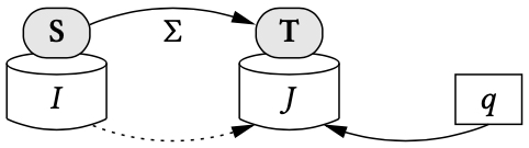
Data exchange is formalized using schema mappings, that is, triples of the form $ℳ=(S,T,\Sigma )$, where $\Sigma$ is a set of constraints that specify the data transformation from $S$ to $T$.¹⁴ If $I$ is a source instance, then a solution for $I$ with respect to $ℳ$ is a target instance $J$ such that the pair $(I,J)$ satisfies the constraints in $\Sigma$. The active domain of $I$ consists entirely of constants, while the active domain of $J$ may contain both constants and labelled nulls. If the schema mapping $ℳ$ is understood from the context, we simply talk about a solution for $I$, instead of a solution for $I$ with respect to $ℳ$.

If $ℳ$ is a schema mapping and $I$ is a source instance, we write $W(ℳ,I)$ to denote the set of all solutions for $I$. In general, the constraints in $\Sigma$ may over-specify or under-specify the data transformation task, hence $W(ℳ,I)$ may be the empty set or a non-empty finite set or an infinite set. If $q$ is a query over the target schema $T$, we can consider the certain answers of $q$ on $W(ℳ,I)$, that is, the set

The pair $(ℳ,I)$ is a compact representation of the space $W(ℳ,I)$ of all solutions for $I$. Thus, the question arises: can this compact representation be used to compute the certain answers of target queries, and if so, how? As shown in,¹⁴ there are many natural settings in which the pair $(ℳ,I)$ is used to compute a universal solution for $I$, a special type of solution for $I$ with the property that the certain answers of every conjunctive query can be obtained by directly evaluating the query on the universal solution.

By a definition, a universal solution for $I$ is a solution $J$ for $I$ such that for every solution $J^{\prime }$ for $J$, there is a homomorphism $h$ from $J$ to $J^{\prime }$ that is the identity on the constants in $J$. Intuitively, a universal solution for $I$ is a “most general” solution for $I$ because it has no more and no less information than what is encapsulated in the pair $(ℳ,I)$. Universal solutions can be used to obtain the certain answers of conjunctive target queries. More precisely, let $ℳ=(S,T,\Sigma )$ be a schema mapping, $I$ a source instance, and $q$ a target conjunctive query. If $J$ is a universal solution for $I$, then $\text{CERTAIN}(q,W(ℳ,I))=q{\left(J\right)}_{\downarrow }$, where $q{\left(J\right)}_{\downarrow }$ is the set of of all null-free tuples of $q\left(J\right)$. The proof follows from the definitions and the fact that conjunctive queries are preserved under homomorphisms.

When do universal solutions exist? To answer this question, we also need to address a different question: what are good schema-mapping specification languages, that is, languages for expressing the constraints used in schema mappings? Ideally, a good schema-mapping specification language should strike a balance between high expressive power and tame computational behavior. From top down, if arbitrary first-order formulas are allowed to specify schema mappings, then it is easy to show that there are simple conjunctive queries for which computing the certain answers is an undecidable problem. From bottom up, let us consider some basic data transformation tasks that every schema-mapping specification language ought to support. In each case, we first describe the transformation and then give a first-order formula expressing an example of it.

• Project out a column from a source relation and copy the result to a target relation; in symbols, $\forall x\forall y\left(P\right(x,y)\to R(x\left)\right)$.

• Decompose a source relation into two target relations; in symbols, $\forall x,y,z\left(P\right(x,y,z)\to R(x,y)\wedge Q(y,z\left)\right)$.

• Add a column to a source relation and copy the result to a target relation; in symbols, $\forall x\left(P\right(x)\to \exists zR(x,z\left)\right)$.

• Join two source relations and copy the result to a target relation; in symbols, $\forall x,y,z\left(E\right(x,y)\wedge F(y,z)\to H(x,y,z\left)\right)$.

The formulas expressing the preceding data transformations are first-order formulas of the form $\forall x\left(\varphi \right(x)\to \exists y\psi (x,y\left)\right)$, where $\varphi \left(x\right)$ is a conjunction of atoms with variables from $x$ and $\psi (x,y)$ is a conjunction of atoms with variables from $x$ and $y$. These formulas are known as tuple-generating dependencies (tgds) and constitute one of the broadest classes of integrity constraints in databases.¹⁵ In fact, the formulas that we used to express these data transformations belong to a special class of tgds called source-to-target tgds (s-t tgds), because the atoms in the antecedent $\varphi \left(x\right)$ of each tgd are over the source schema, while the atoms in the consequent $\psi (x,y)$ are over the target schema.

In what follows, we will consider schema mappings $ℳ=(S,T,\Sigma )$ where $\Sigma$ always contains s-t tgds. In addition, $\Sigma$ may include target tgds and target equality-generating dependencies (target egds). Target tgds are tgds of the form $\forall x\left(\varphi \right(x)\to \exists y\psi (x,y\left)\right)$ in which both $\varphi \left(x\right)$ and $\psi (x,y)$ are conjunctions of atoms over the target schema; target egds are first-order formulas of the form $\forall x(\varphi \left(x\right)\to x_i=x_j)$, where $\varphi \left(x\right)$ is a conjunction of atoms over the target schema and $x_i,x_j$ are two distinct variables from $x$. Target tgds and target egds are the most extensively studied class of integrity constraints over a database schema.¹⁵ As special cases, they contain the functional dependencies and the full tgds, which are tgds with no existential quantifiers in the consequent.

Let $ℳ=(S,T,\Sigma )$ be a schema mapping and let $q$ be a Boolean target conjunctive query.

• The existence-of-universal-solutions problem $\mathrm{EoU}\left(ℳ\right)$ asks: given a source instance $I$, is there a universal solution $J$?

• The certain answers problem $\text{C}\text{ERTAINTY}(q,ℳ)$ asks: given a source instance $I$, is $\text{CERTAIN}(q,W(ℳ,I\left)\right)$ true?

The complexity of these two decision problems exhibits diverse behavior, which depends on the constraints allowed in the schema mappings. Figure 3 summarizes the precise results in three parts. Next, we discuss the main ideas behind the proofs of each part.

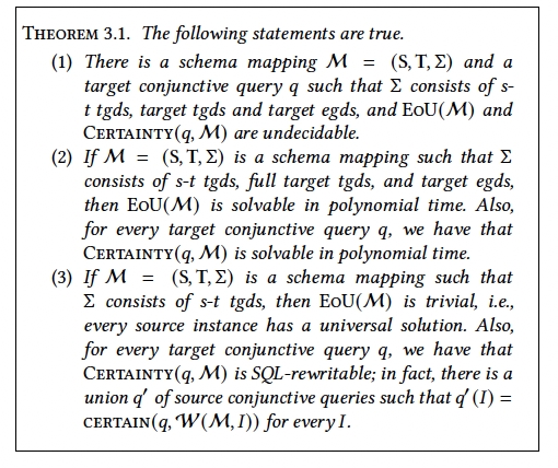
The undecidability results in the first part are obtained via a reduction from the embedding problem for finite semigroups: given a finite partial semigroup, can it be extended to a finite semigroup? (see Kolaitis et al.²⁴ for the details).

The main tool for the tractability results in the second part is the chase procedure, a versatile algorithm originally designed to study the implication problem for database dependencies.^2,7,29 Intuitively, when an instance is chased with a set of tgds and egds, we consider all instantiations of variables that satisfy the antecedents of the constraints and then generate new facts as needed to satisfy the consequents of the constraints. For example, if the instance consists of the fact $E(1,2)$ and is chased with the tgd $\forall x,y\left(E\right(x,y)\to \exists z(H(x,z)\wedge H(z,y))$, then the chase procedure will generate a labelled null $N_i$ and the facts $H(1,N_i)$ and $H(N_i,2)$. With egds, the chase will attempt to equate the values of the two variables in the consequent of the egd by replacing a labelled null by a constant or one labelled null by another, but it will fail if it has to equate two different constants.

In general, the chase procedure may not terminate. There are, however, broad sufficient conditions guaranteeing the termination of the chase. In particular, if the set of the target tgds in the schema mapping considered obeys certain structural conditions, such as weak acyclicity, then the chase procedure terminates within time bounded by a polynomial in the size of the input structure and produces a universal solution precisely when a solution exists.¹⁴ Every set of full tgds is weakly acyclic, while the set consisting of the target tgd $\forall x,y\left(H\right(x,y)\to \exists zH(y,z\left)\right)$ is not. Actually, if the instance consisting of the fact $H(1,2)$ is chased with this tgd, then the chase procedure will not terminate as it will generate an infinite sequence $H(2,N_1),H(N_1,N_2),H(N_2,N_3),\dots$ of facts.

As regards the rewritability results in the third part, if a schema mapping $ℳ=(S,T,\Sigma )$ is specified using s-t tgds only, then, given a source instance $I$, the chase procedure always terminates and produces a universal solution $J$ for $I$ in time bounded by a polynomial in the size of $I$. Therefore, by the properties of universal solutions. $J$ can be used to compute the certain answers $\text{CERTAIN}(q,W(ℳ,I\left)\right)$, where $q$ is a target conjunctive query, in time bounded by a polynomial in the size of $I$. In this case, however, the certain answers can also be obtained by rewriting $q$ to a union $q^{\prime }$ of conjunctive queries over the source schema and then directly evaluating $q^{\prime }$ on $I$. This is achieved by “decomposing” $\Sigma$ into a set of local-as-view (LAV) constraints and a set of global-as-view (GAV) constraints, where a LAV constraint is a tgd whose antecedent consists of a single atom and a GAV constraint is a tgd whose consequent consists of a single atom. The rewriting of $q$ into $q^{\prime }$ can then be achieved by combining the MiniCon algorithm for LAV constraints³¹ with an unfolding technique for GAV constraints.

For further reading about data exchange, see the monograph⁵ and the collection.²⁴

Inconsistent Databases

In designing databases, one specifies a schema $S$ and a set $\Sigma$ of integrity constraints on $S$. An inconsistent database is a database $I$ that does not satisfy $\Sigma$. Inconsistent databases arise in a variety of contexts and for different reasons, including the following two. First, a database system may not support the enforcement of a particular type of integrity constraints. Second, data at different sources may be transferred to a central repository and the resulting database may be inconsistent, even though each source database is consistent.

The framework of database repairs, introduced by Arenas, Bertossi, and Chomicki,⁵ is a principled approach to coping with inconsistent databases and without “cleaning” dirty data first. Database repairs constitute a mechanism for representing possible worlds through interventions in the database. Specifically, given an inconsistent database, the aim is to achieve consistency through some minimal intervention in the database. There may exist, however, many different such minimal interventions, and it may not be known which one represents the ground truth. Hence, the result of each such minimal intervention is viewed as a possible world.

Let $\Sigma$ be a set of integrity constraints and let $I$ be an inconsistent database. Intuitively, a database $J$ is a repair of $I$ w.r.t. $\Sigma$ if $J$ is a consistent database (that is, $J\vDash \Sigma$), and $J$ differs from $I$ in a “minimal” way. Several different types of repairs have been considered, including set-based repairs (subset, superset, $\oplus$-repairs), cardinality-based repairs, attribute-based repairs, and preferred repairs.

In what follows, we will focus on subset repairs and so from now on we will use the term repair, instead of the term subset repair.

A straightforward generalization of this example shows that an inconsistent database may have exponentially many repairs.

The consistent answers are certain answers, where the possible worlds are the repairs. Indeed, if $\Sigma$ is a set of constraints and $I$ is a database, let $W\left(I\right)$ be the set of all repairs of $I$ w.r.t. $\Sigma$. Then $\text{C}\text{ONS}(q,I,\Sigma )=\text{CERTAIN}(q,W(I\left)\right)$.

Let us revisit the preceding Example 4.2, where we have:

• If $q\left(x\right)$ is the query $\exists yR(x,y)$, then $\text{C}\text{ONS}(q,I,\Sigma )=\{a_1,a_2\}.$

• If $q\left(x\right)$ is the query $\exists zR(z,x)$, then $\text{C}\text{ONS}(q,I,\Sigma )=\varnothing .$

Let $\Sigma$ be a set of integrity constraints and let $q$ be a Boolean query. $\text{C}\text{ERTAINTY}(q,\Sigma )$ is the following decision problem: Given a database $I$, is $\text{C}\text{ONS}(q,I,\Sigma )$ true? (In other words, is $q$ true on every repair of $I$?) We will examine the complexity of $\text{C}\text{ERTAINTY}(q,\Sigma )$ in a basic setting, namely, when $q$ is a Boolean conjunctive query and $\Sigma$ is a set of key constraints with one key per relation.

We first observe that in this setting the repair-checking problem w.r.t. $\Sigma$ is in $\text{P}$, where this problem asks: given two databases $I$ and $J$, is $J$ a repair of $I$ w.r.t. $\Sigma$? From this observation and the relevant definitions, it follows that if $\Sigma$ is a set of key constraints with one key constraint per relation and $q$ is a Boolean conjunctive query, then $\text{C}\text{ERTAINTY}(q,\Sigma )$ is in $\mathrm{coNP}$.

Let $\Sigma$ be the following set of constraints asserting that the binary relations $R$ and $S$ have their first attribute as key:

Consider the following two Boolean queries:

• $q_1$ is the path query $\exists x,y,z\left(R\right(x,y)\wedge S(y,z\left)\right)$.

• $q_2$ is the sink query $\exists x,y,z\left(R\right(x,y)\wedge S(z,y\left)\right)$.

The question now arises: what can we say about the computational complexity of $\text{C}\text{ERTAINTY}(q_i,\Sigma )$, $i=1,2$? Fuxman and Miller¹⁷ showed that $\text{C}\text{ERTAINTY}(q_1,\Sigma )$ is in $\text{P}$, whereas $\text{C}\text{ERTAINTY}(q_2,\Sigma )$ is $\mathrm{coNP}$-complete.

We first explain why $\text{C}\text{ERTAINTY}(q_1,\Sigma )$ is in $\text{P}$. In fact, a stronger result holds: $\text{C}\text{ERTAINTY}(q_1,\Sigma )$ is FO-rewritable, which means that there is a first-order definable query $q^{*}$ such that for every database $I$, we have $\text{C}\text{ONS}(q_1,I,\Sigma )$ is true if and only if $q^{*}\left(I\right)$ is true.

Concretely, it is easy to verify that $q^{*}$ is the query

From a complexity standpoint, FO-rewritability is the most desirable outcome: we can compute the consistent answers by directly evaluating a FO-query on the inconsistent database. Furthermore, FO-rewritability implies that $\text{C}\text{ERTAINTY}(q_1,\Sigma )$ is in $\text{P}$.

Next, we show that $\text{C}\text{ERTAINTY}(q_2,\Sigma )$ is $\mathrm{coNP}$-complete via a polynomial-time reduction from the (complement of) Monotone SAT, which is the restriction of SAT to monotone formulas, that is, to Boolean formulas in conjunctive normal form such that each clause (conjunct) of the formulas is either a disjunction of variables (positive clause) or a disjunction of negated variables (negative clause).

Given a monotone formula $\varphi$, construct a database $I$ with relations $R$ and $S$: if $c$ is a positive clause and the variable $v$ occurs in $c$, then put $(c,v)$ in $R$; if $c$ is a negative clause and $v$ occurs in $c$, then put $(c,v)$ in $S$. It is now easy to verify that $\varphi$ is satisfiable if and only if $\text{C}\text{ONS}(q_2,I,\Sigma )$ is false (that is, there is a repair $J$ of $I$ such that $q\left(J\right)$ is false). Thus, $\text{C}\text{ERTAINTY}(q_2,\Sigma )$ is $\mathrm{coNP}$-complete.

Next, consider the following Boolean query:

• $q_3$ is the cycle query $\exists x,y\left(R\right(x,y)\wedge S(y,x\left)\right)$.

Wijsen³⁶ showed that $\text{C}\text{ERTAINTY}(q_3,\Sigma )$ is in $\text{P}$, but it is not FO-rewritable. Thus, FO-rewritability is not the only way in which the consistent answers of a query can be tractable.

In summary, we have seen that the following statements are true.

• $\text{C}\text{ERTAINTY}(q_1,\Sigma )$ is in $\text{P}$; in fact, it is FO-rewritable.

• $\text{C}\text{ERTAINTY}(q_3,\Sigma )$ is in $\text{P}$, but it is not FO-rewritable.

• $\text{C}\text{ERTAINTY}(q_2,\Sigma )$ is $\mathrm{coNP}$-complete.

The trifurcation in the complexity of $\text{C}\text{ERTAINTY}(q_i,\Sigma )$, for $i=1,2,3$, is not an isolated phenomenon, but an instance of a deeper result, depicted in Figure 4, about conjunctive queries without self-joins. In that result, the boundaries of the trichotomy are delineated with the help of a graph, called the attack graph, which is associated with $\Sigma$ and $q$. This graph has two types of edges, regular edges and strong edges. If the attack graph is acyclic, then $\text{C}\text{ERTAINTY}(q,\Sigma )$ is FO-rewritable. If the attack graph is cyclic, but no cycle contains a strong edge, then $\text{C}\text{ERTAINTY}(q,\Sigma )$ is in $\text{P}$ but it is not FO-rewritable. Finally, if the attack graph has a cycle containing at least one strong edge, then $\text{C}\text{ERTAINTY}(q,\Sigma )$ is coNP-complete.

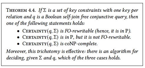
The Koutris-Wijsen Dichotomy Theorem vastly generalizes several different earlier dichotomy results, including the one in²⁵ that classifies the queries that consist of two atoms over two distinct relations. The classification of the complexity of $\text{C}\text{ERTAINTY}(q,\Sigma )$ for arbitrary Boolean conjunctive queries (including those with self-joins) remains an open problem.

For further reading about inconsistent databases and consistent answers, see the monograph.⁸

Probabilistic Databases

A probabilistic database is a probability space over possible worlds (that is, ordinary databases). Restricting to the discrete case, which is the most commonly studied, we formally define a probabilistic database over a schema $S$ as a pair $(P,p)$ where $P$ is a countable set of databases over $S$, and is, ${\sum }_{J\in P}p\left(J\right)=1$. The conventional semantics of query evaluation over a probabilistic database asks for the marginal probability of every answer. For a Boolean query, this amounts to computing the probability that the query is true on a random possible world. Formally, the task is to compute the probability $\mathrm{Pr}\left[q\right]$ that $J\vDash q$ when $J$ is drawn randomly from $(P,p)$:

As conventional in probabilistic modeling, we seek compact representations of probabilistic databases, where a finite object represents many possible worlds (for example, exponential number w.r.t. the size of the representation itself). Such representations rely on assumptions of probabilistic independence that, in turn, allow for factorization. The most studied representation is the Tuple-Independent Database (TID)¹¹ (with roots in prior work, for example, Grädel et al.¹⁹). A TID is represented as an ordinary database where each fact is associated with a probability of existence. Then, a possible world is a subset of the database and it is randomly drawn by independently considering each tuple and deciding whether or not it is valid. More formally, a TID over a schema $S$ is represented as a pair $(I,\pi )$ where $I$ is a database over $S$ and $\pi :I\to [0,1]$ assigns a probability to each fact. The pair $(I,\pi )$ represents the probabilistic database $(P,p)$ where $P$ consists of all the subsets of $I$ and

The computational complexity of query evaluation over TIDs has been scrutinized by the database community over the past two decades. As we shall see next, the probability of a query can be $\#P$-hard even for very simple join queries. Past results have established thorough classifications of query classes into tractable and intractable, in either the exact or approximate sense. In this part, we explain the first dichotomy found for TIDs¹¹ that considers the class of conjunctive queries without self-joins. We refer to it as the Little Dichotomy Theorem as it was later generalized to the broader class of all union of conjunctive queries (or, equivalently, the class of queries that can be phrased using the positive operators of the relational algebra).¹²

Before we give the dichotomy, let us illustrate it. For the positive side, let $q_1$ be the query $\exists x\exists y\left(R\right(x)\wedge S(x,y)$. Given the input TID $(I,\pi )$, we compute $\mathrm{Pr}\left[q\right]$ as follows. First, write $q_1$ as $\exists x\left(R\right(x)\wedge \exists yS(x,y\left)\right)$. Then, using tuple-independence, we have that:

The last expression has size $O\left(n^2\right)$, where $n=\left|\mathrm{dom}\right(I\left)\right|$.

An example of an intractable query is $\exists x\exists y\left(R\right(x)\wedge S(x,y)\wedge T(y\left)\right)$, which we denote by $q_2$. We will show that $\mathrm{Pr}\left[q_2\right]$ is $\#P$-complete through a reduction from a well known $\#P$-complete problem.

A positive partitioned 2DNF formula (PP2DNF) is a DNF-formula of the form $(x_{i_1}\wedge y_{j_1})\vee \cdots \vee (x_{i_k}\wedge y_{j_k}),$ where the $x_i$’s and the $y_j$’s form disjoint sets of variables. Counting the satisfying assignments of a PP2DNF formula known to be $\#P$-complete.³² We can visualize a PP2DNF as a bipartite graph, where the left and right sides consist of the $x$ and $y$ variables, respectively, and the edges correspond to the clauses. As an example, the graph of Figure 5a corresponds to the formula $(x_1\wedge y_1)\vee (x_1\wedge y_2)\vee (x_2\wedge y_1)$. If we view a truth assignment to the variables as stating whether a vertex is present or not, then a satisfying assignment corresponds to a non-independent set, that is, a set of vertices with at least one edge. Hence, the number of satisfying assignments is $2^n–M$ where $n$ is the number of variables and $M$ is the number of independent sets. Also, every bipartite graph represents some PP2DNF formula in this way. Thus, counting the satisfying assignments of a PP2DNF formula is the same as counting the independent sets of a bipartite graph.

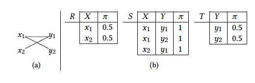
Dalvi and Suciu¹¹ showed that this problem can be simulated as the evaluation of $q_2$ over a TID, as we illustrate in Figure 5a. Let $(I,\pi )$ be the TID shown in Figure 5b. There is a one-to-one correspondence between truth assignments for $\varphi$ and possible worlds for $(I,\pi )$. The reader can easily verify that $\#\varphi =2^n\mathrm{Pr}\left[q_2\right]$ where $n$ is the number of variables of $\varphi$. Hence, we reduce #PP2DNF to $\mathrm{Pr}\left[q_2\right]$.

The queries $q_1$ and $q_2$ are examples of hierarchical and non-hierarchical queries, respectively. As it turns out, the property of being hierarchical characterizes tractability. A conjunctive query $q$ without self-joins is hierarchical if for every two variables $x$ and $y$ of $q$, either $\mathrm{at}\left(x\right)\subseteq \mathrm{at}\left(y\right)$, or $\mathrm{at}\left(y\right)\subseteq \mathrm{at}\left(x\right)$, or $\mathrm{at}\left(x\right)\cap \mathrm{at}\left(y\right)=\varnothing$, where $\mathrm{at}\left(z\right)$ is the set of all atoms of $q$ where $z$ appears.

For example, our query $q_1$, namely $\exists x\exists y\left(R\right(x)\wedge S(x,y\left)\right)$, is hierarchical, since $\mathrm{at}\left(y\right)\subseteq \mathrm{at}\left(x\right)$. Query $q_2$, namely $\exists x\exists y\left(R\right(x)\wedge S(x,y)\wedge T(y\left)\right)$, is not hierarchical since $at\left(x\right)\cancel{\subseteq }at\left(y\right)$, $at\left(y\right)\cancel{\subseteq }at\left(x\right)$, and yet, $\mathrm{at}\left(x\right)$ and $\mathrm{at}\left(y\right)$ have a common member, namely $S(x,y)$.

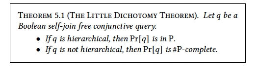
Figure 6 depicts the formal theorem that we refer to as the “little dichotomy theorem,” stating that being hierarchical characterizes being tractable (under standard complexity assumptions) as far as conjunctive queries without self-joins are concerned.

For further reading about probabilistic databases, we refer the reader to the monograph.³⁴

Election Databases

Social choice theory is concerned with the aggregation of individual preferences into a collective outcome. Election databases form a framework that infuses social choice theory with relational database context. An election database may contain information about individual candidates (for example, age, education, wealth), voters (for example, age, occupation, affiliation), positions of candidates on various issues, and preferences of voters. This framework supports the formulation of sophisticated queries that go well beyond asking who the winners in some election are, which is the traditional focus of social choice theory. Ideally, each voter casts a complete preference, which is formalized as a total order of the candidates that the voter has to rank. It is often the case, however, that some voters can only cast incomplete preferences, which are formalized as partial orders of the candidates. Each such partial order represents the possible total rankings of the candidates by a voter, and different total rankings may produce different election outcomes. This constitutes a different mechanism for defining possible worlds.

To present a more rigorous treatment, we first recall the basic terminology of voting theory in computational social choice; for additional background, we refer the reader to the Handbook of Computational Social Choice.¹⁰ Let $C=\{c_1,\dots ,c_m\}$ be a set of candidates, and let $V=\{v_1,\dots ,v_n\}$ be a set of voters. A complete voting profile is a tuple $T=(T_1,\dots ,T_n)$, where each $T_i$ is a total order over $C$, representing the ranking (preference) of voter $v_i$ of the candidates in $C$. A voting rule $r$ is a function that maps every complete profile $T$ into a set $W(r,T)\subseteq C$ of winners. We say that a candidate $c$ is a winner if $c\in W(r,T)$.

We focus on the class of positional scoring rules, which is arguably the most extensively studied class of voting rules in computational social choice. A positional scoring rule $r$ maps every number $m$ of candidates to a scoring vector $\left(r\right(m,1),\cdots ,r(m,m\left)\right)$ of natural numbers where $r(m,1)\ge r(m,2)\dots \ge r(m,m)$. Here, $r(m,j)$ is the score that a candidate is awarded when positioned $j$th by a voter. The score $s(T_i,c)$ of a candidate $c$ on the order $T_i$ of the voter $v_i$ is $r(m,j)$, where $j$ is the position of candidate $c$ in $T_i$. When $r$ is applied to $T=(T_1,\dots ,T_n)$, it assigns to each candidate $c$ the sum ${\sum }_{i=1}^{n}s(T_i,c)$ as the score of $c$. A candidate is a winner if her score is greater or equal to the score of every candidate. Popular positional scoring rules include the plurality rule $(1,0,\cdots ,0)$ where the winners are the candidates most frequently ranked first, the veto rule $(1,\cdots ,1,0)$ where the winners are the candidates least frequently ranked last, and the Borda rule $(m–1,m–2,\cdots ,0)$, where the score of a candidate is the position itself minus 1 in reverse order.

To avoid trivialities, we assume that every $r(·,m)$ contains at least two different score values, that is, $r(m,1)>r(m,m)$. We also assume that the scores in $r(·,m)$ are co-prime (that is, their biggest common divisor is 1), since multiplying all scores by the same number has no impact on the outcome. Rule $r$ is pure if for every $m\ge 2$, the scoring vector $r(·,m)$ is obtained from $r(·,m–1)$ by inserting a score value at some position. For example, essentially all specific rules studied in the literature (for example, plurality, veto and Borda) are pure.

A partial voting profile is a tuple $P=(P_1,\dots ,P_n)$, where each $P_i$ is a partial order over the set $C$ of candidates, representing a partially known preference of the voter $v_j$. A completion of $P=(P_1,\dots ,P_n)$ is a complete voting profile $T=(T_1,\dots ,T_n)$ such that each $T_i$ is a completion of $P_i$, that is, a total order that completes the partial order $P_i$. A candidate $c$ is a necessary winner if $c\in W(r,T)$ for all completions $T$.²⁶ (We later discuss the analogous notion of a possible winner.)

An election database consists of a partial voting profile, along with a database $I$ that has contextual information about the candidates. Formally, it is a tuple $(I,C,P,r)$ that represents a set of possible worlds, where each possible world is a completion of $I$. In turn, a completion of $I$ is obtained by taking a completion $T$ of $P$, and adding to $I$ a new unary relation $\text{W}\text{INNER}$ that has the fact $\text{W}\text{INNER}\left(c\right)$ for each winner $c\in W(r,T)$. In particular, the possible worlds are identical, except for the content of the $\text{W}\text{INNER}$ relation that depends on the underlying completion of $P$. A Boolean query $q$ is necessary if $J\vDash q$ for all completions $J$ of $I$. (Note that “necessary” is the adaptation of the term “certain” to the election setting.)

As an example, let $c$ be a candidate and $q$ be the query $\text{W}\text{INNER}\left(c\right)$. Then $q$ is necessary if and only if $c$ is a necessary winner. As another example, let $q^{\prime }$ be the query $\exists x\left[\text{W}\text{INNER}\right(x)\wedge R(x\left)\right]$ where $R$ can be thought of as representing a party of candidates. Necessity of $q^{\prime }$ means that there is necessarily a winner from $R$. Note that it may be the case that $q$ is necessary even if no candidate in $R$ is a necessary winner, and even if there are no necessary winners at all.

We now discuss the problem of deciding the necessity of a Boolean conjunctive query $q$ under a positional scoring rule $r$. This problem has two parameters, $q$ and $r$, and the input consists of a candidate set $C$, a partial profile $P$, and a database $I$.

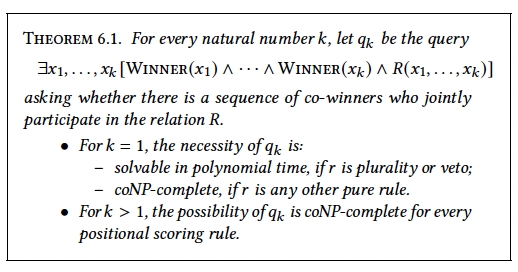
An immediate observation is that the necessity problem is in coNP. Let us consider several examples of tractability and hardness. The simplest example is the query $\exists x\left[\text{W}\text{INNER}\right(x\left)\right]$ asking whether there exists a winner. By definition, there is always one or more winners, so this query is necessary on every election database (and the problem is trivially solvable in constant time). More interesting examples are the conjunctive queries depicted in Figure 7, namely,

for different $k\ge 1$, asking whether there are $k$ winners who participate in the $k$-ary relation $R$. In the remainder of this section, we discuss the proofs of the complexity results in Figure 7.

We begin with $k=1$. In the case of plurality and veto, the polynomial-time algorithm is based on a polygamous version of the perfect-matching problem, where each vertex of one side should be matched with a number of neighbors from the other side, and this number is from an interval associated to the vertex. Hardness for the remaining pure rules is via a reduction from the problem of the possible unique winner: given a partial profile $P$ and a member $c$ of the set $C$ of candidates, is there any completion where $c$ is the single winner? Indeed, the complexity of this problem exhibits a classification analogous to the theorem: it is solvable in polynomial time under plurality and veto, yet NP-hard for every other pure rule.⁶

For $k=2$, hardness for plurality and veto is proved via the maximum independent set problem, and hardness for any other pure rule is via a reduction from $k=1$. Hardness for $k>2$ can be easily established via a reduction from $k=2$. Interestingly, Kimelfeld et al.²² used a more complex reduction (from DNF tautology) that applies to all positional scoring rules, pure or not; hence, for $k>2$ the necessity problem is coNP-complete for every such rule.

We conclude this section with several comments. First, in the case of the plurality rule, a dichotomy in the complexity has been establish for a large fragment of conjunctive queries.²¹ Second, the necessity problem becomes tractable if we assume that the number of candidates is small. In particular, the problem is fixed-parameter tractable with respect to the parameter $\left|C\right|$ for every polynomial-time query.²²

Concluding Remarks

The possible world semantics is a natural and principled approach to coping with deficiencies in data. We discussed the versatility of this approach in such deficiencies as missing information (null values), under-specified transformations (data exchange), violation of integrity constraints (inconsistent databases), and quantified uncertainty (probabilistic databases). When possible world semantics is adopted, query evaluation entails the aggregation of the results of the query over the possible worlds. The intersection of the results (certain/consistent answers) amounts to logical inference—these are the answers that are derived from the deficient data. Summation in probabilistic databases amounts to probabilistic inference—each answer is assigned its marginal probability. Other aggregation mechanisms have also been investigated. We touched on the union (possible answers) in passing, but did not cover the range semantics for queries with numerical operators, such as COUNT and SUM.⁵ There is also work on combinations of settings discussed here; relevant references are given in the online appendix.

The adoption of the possible world semantics increases the computational complexity since the number of possible worlds can be prohibitively large. Indeed, computational hardness already arises for frequently asked queries, such as conjunctive queries; we discussed several dichotomy theorems that strive to delineate the boundary between tractability and intractability for queries in a class. In practice, however, hard problems are often attacked by general-purpose tools, such as integer linear programming, SAT solvers, and answer-set programming, as done in consistent query answering,^13,24 variants of consistent query answering^9,30, and probabilistic databases.^16,33

Beyond data management, the possible world semantics provides a natural approach to incorporating contextual data in the study of other settings that involve deficiencies. As a case in point, we illustrated this idea by discussing the framework of election databases. We believe that the versatility of the possible world semantics can have significant applications in a plethora of other fields.