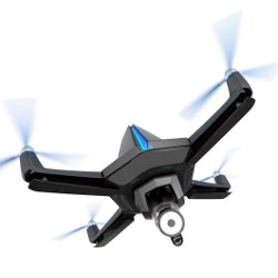
Autonomous drones represent a new breed of mobile computing system. Compared to smartphones and connected cars that only opportunistically sense or communicate, drones allow motion control to become part of the application logic. The efficiency of their movements is largely dictated by the low-level control enabling their autonomous operation based on high-level inputs. Existing implementations of such low-level control operate in a time-triggered fashion. In contrast, we conceive a notion of reactive control that allows drones to execute the low-level control logic only upon recognizing the need to, based on the influence of the environment onto the drone operation. As a result, reactive control can dynamically adapt the control rate. This brings fundamental benefits, including more accurate motion control, extended lifetime, and better quality of service in end-user applications. Based on 260+ hours of real-world experiments using three aerial drones, three different control logic, and three hardware platforms, we demonstrate, for example, up to 41% improvements in motion accuracy and up to 22% improvements in flight time.
1. Introduction
Robot vehicle platforms, often called “drones,” offer exciting new opportunities for mobile computing. While many mobile systems, such as smartphones and connected cars, simply respond to device mobility, drones allow computer systems to actively control device location. Such a feature enables interactions with the physical world to happen in new ways and with new-found scale, efficiency, or precision.4,8,18
Autopilots. Figure 1 schematically illustrates the hardware and software components in modern drone platforms. Key to their operation is the autopilot software implementing the low-level motion control. The control loop processes high-level commands coming from a Ground-Control Station (GCS) as well as various sensor inputs, such as, accelerations and Global Positioning System (GPS) coordinates, to operate actuators such as electrical motors that set the 3D orientation of the drone.

Figure 1. Hardware and software components in modern drone platforms. Users configure high-level mission parameters at the ground-control station (GCS), whereas the autopilot software implements the low-level motion control aboard the drone.
Together with the mechanical design, the autopilot software is crucial to determine a drone’s performance along a number of essential metrics. For example, the low-level control directly influences the quality of the shots when using drones for imagery applications.17, 18 Further, it is partly responsible for the overall energy efficiency, as a drone’s lifetime is often a result of how streamlined is the autopilot operation.5, 24
Unsurprisingly, most existing autopilots employ Proportional-Integral-Derivative (PID)2 designs. Processing is thus time-triggered: every T time units, sensors are probed, control decisions are computed, and commands are sent to the actuators. Such a deterministic operation simplifies implementations and allows designers to directly rely on a vast body of existing literature.2
Reactive control. Based on a handful of key observations, a fundamental leap of abstraction, and an unconventional use of recent advances in programming languages, we conceive a notion of reactive control that allows autopilots to significantly improve a drone’s performance in both motion accuracy and energy consumption. Rather than periodically triggering the control logic, we only run the control logic upon recognizing the need to. Depending on the influence of the environment onto the drone operation, for example, due to wind gusts or pressure gradients, control may run more or less frequently, regardless of the the fixed rate of a corresponding time-triggered implementation. As a result, reactive control dynamically adapts the control rate.
Reactive control yields several advantages, including more timely and adaptive control decisions leading to improved motion accuracy and energy efficiency. As it exclusively works in software, reactive control also requires no hardware modifications. We provide concrete evidence of these benefits across different aerial drone applications, based on 260+ hours of test flights in three increasingly demanding environments, using a combination of three aerial drones, three autopilot software, and three embedded hardware platforms. Our results indicate, for example, that reactive control obtains up to 41% improvements in the accuracy of motion, and up to a 22% extension of flight times.
The remainder of the paper unfolds as follows. Section 2 provides the necessary background, elaborates on the fundamental intuitions behind reactive control, and outlines the issues that are to be solved to make it happen. Section 3 describes the specific techniques we employ to address these issues. Section 4 reports on the performance of reactive control compared with traditional time-triggered implementations, whereas Section 5 studies the impact of reactive control in a paradigmatic end-user application. We conclude the paper in Section 6 by discussing our current work towards obtaining official certifications to fly drones running reactive control over public ground.
2. Building up to Reactive Control
Reactive control relies on concepts and techniques germane to statistics, embedded software, programming languages, control, and low-power hardware. In the following, we try and smooth the waters for the readers by walking them through the characteristics of target platforms, the key observations leading to reactive control, and the issues that are to be solved to concretely realize it.

Drones can be regarded as a cruder form of modern robotics.9 The high-level inputs coming from the GCS may be a waypoint or a trajectory. Autopilots implement the low-level control in charge of translating these inputs into commands for the drone actuators.
Ardupilot (goo.gl/x2CHyM) is an example autopilot implementation, providing reliable low-level control for aerial drones and ground robots. The project boasts a large on-line community and is at the basis of many commercial products.
Software. Figure 2 shows the execution of Ardupilot’s low-level control loop, split in two parts. The fast loop only includes critical motion control functionality. The time left from the execution of fast loop is given to an application-level scheduler that distributes it among non-critical tasks that may not always execute, such as logging. The scheduler operates in a best-effort manner based on programmer-provided priorities. Many autopilots share similar designs.7

Figure 2. Ardupilot’s low-level control loop. The time for a single iteration of the loop is split between fast loop, which only includes critical motion control functionality, and an application-level scheduler that runs non-critical tasks.
Initially, fast loop blocks waiting for a new value from the Inertial Measurement Unit (IMU). This provides an indication of the forces the drone is subject to, obtained by combining the readings of accelerometers, gyroscopes, magnetometers, and barometer. Once a new value is available, IMU information is combined with GPS readings to determine how the motors should operate to minimize the error between the desired and actual pitch, roll, and yaw, shown in Figure 3. Multiple PID controllers inside fast loop are used to this end.

Figure 3. Control based on raw, pitch, and yaw.
In Ardupilot as well as the vast majority of autopilots, the control rate is statically set to strike a reasonable tradeoff between motion accuracy and resource consumption, based on a few “rules of thumbs.”6,25 For example, Ardupilot runs at a fixed 400Hz on the hardware we describe next. This rate is not necessarily the maximum the hardware supports. The 400Hz of Ardupilot, for example, are thought to leave enough room—on average—to the scheduler. In short bursts, control may run much faster than 400Hz, as long as some processing time is eventually allocated to the scheduler.
Hardware. Autopilots typically run on resource-constrained embedded hardware, for reasons of size and cost. A primary example is the Pixhawk family of autopilot boards (goo.gl/wU4fmk), which feature a Cortex M4 core at 168MHz and a full sensor array for navigation, including a 16-bit gyroscope, a 14-bit accelerometer/magnetometer, a 16-bit 3-axis accelerometer/gyroscope, and a 24-bit barometer. Most often, at least a sonar and a GPS are added to provide positioning and altitude information, respectively.
Interestingly, the sensors on Pixhawk have similar capabilities as those on modern mobile phones. In fact, many argue that without the push to improve sensors due to the rise of mobile phones, drone technology would have not emerged.9 Such sensors support energy-efficient high-frequency sampling and often provide interrupt-driven modes to generate a value upon verifying certain conditions. The ST LSM303D mounted on the Pixhawk, for example, can be programmed to generate an Serial Peripheral Interface (SPI) interrupt based on three thresholds. This is useful, for example, in human tracking applications for functionality such as fall detection.15
Through our continuous work with drones as mobile computing platforms,16, 19 we eventually noticed that the autopilots’ PID controllers are mostly tuned so that it is the Proportional component to dictate the actual controller operation. The Derivative component can be kept to a minimum though a careful distribution of weights,6, 11 whereas precise sensor calibration may spare the Integral component almost completely.6, 11, 22
As a result of this observation, we concluded that a simple relation exists between current inputs from the navigation sensors and the corresponding actuator settings. With little impact from the time-dependent Derivative and Integral components, and with the Proportional component dominating, small variations in the current sensor inputs likely correspond to small variations in the actuator settings. As an extreme case, as long as the sensor inputs do not change, the actuator settings should remain almost unaltered. In such a case, at least in principle, one may not run the control logic and simply retain the previous actuator settings.
Reactive control builds upon this intuition. We constantly monitor the navigation sensors to understand when the control logic does need to run as a function of the instantaneous environment conditions. These manifest as changes in the inputs of navigation sensors. If these are sufficiently significant to warrant a change in the physical drone behavior to be compensated, reactive control executes the control logic to compute new actuator settings. Otherwise, reactive control retains the existing configuration.
As we explain next, reactive control abstracts the problem of recognizing such significant changes in a way that makes it computationally tractable with little processing resources. Moreover, because of the aforementioned characteristics of sensor hardware on autopilot boards, monitoring the sensor readings at the maximum possible rate usually bears very little energy overhead. Reactive control, nonetheless, makes it possible to rely on the low-power interrupt-driven modes if available.
As a result, when sensor inputs change often, reactive control makes control run repeatedly, possibly at rates higher than the static settings of a time-triggered implementation. When sensor inputs exhibit small or no variations, the rate of control execution reduces, freeing up processing resources that may be needed at different times.
Realizing reactive control is, however, non-trivial. Three issues are to be solved, as we illustrate in Section 3:
- What is a “significant” change in the sensor input depends on several factors, including the accuracy of sensor hardware, the physical characteristics of the drone, the control logic, and the granularity of actuator output. We opt for a probabilistic approach to tackle this problem, which abstracts from all these aspects by employing a form of auto-tuning of the conditions leading to running the control logic.
- An indication for running the control logic may originate from different sensors, at different rates, and asynchronously with respect to each other. A problem is thus how to handle the possible inter-leavings. Moreover, not running the control loop for too long may negatively affect the drone’s stability, possibly preventing to reclaim the correct behavior. We tackle these issues by only changing the execution of the control logic over time, rather than the logic itself.
- Reactive control must run on resource-constrained embedded hardware. When implementing reactive control, however, the code quickly turns into a “callback hell”10 as the operation becomes inherently event-driven. We experimentally find that, using standard languages and compilers, this negatively affects the execution speed, thus limiting the gains.7 We design and implement a custom realization of Reactive Programming (RP) techniques3 to tackle this problem.
The context where we are to address these issues shapes the challenge in unseen ways. For example, aerial drone demonstrations exist showing motion control in tasks such as throwing and catching balls,21 flying in formation,23 and carrying large payloads.14 In these settings, the low-level control does not operate aboard the drone. At 100Hz or more, a powerful computer receives accurate localization data from high-end motion capture systems, runs sophisticated control algorithms based on drone-specific mechanical models expressed through differential equations, and sends actuator commands to the drones. Differently, we aim at improving the performance of mainstream low-level control on embedded hardware, targeting mobile sensing applications that operate in the wild.
On the surface, reactive control may also resemble the notion of event-based control.1 Here, however, the control logic is often expressly redesigned for settings different than ours; for example, in distributed control systems to cope with limited communication bandwidth or unpredictable latency. This requires a different theoretical framework.1 In contrast, we aim at re-using existing control logic, whose properties are well understood, and at doing so with little or no knowledge of its corresponding implementation and its parameter tuning. Different than event-based control, in addition, reactive control is mainly applicable only to PID-like controllers where the Proportional component dominates.
3. Reactive Control
The key issues we discussed require dedicated solutions, as we explain here.
Problem. It may seem intuitive that the more “significant” is a change in a sensor reading, the more likely is the necessity to run the control loop. Such a condition would indicate that something just happened in the environment that requires the drone to react. However, what is a “significant” change in the sensor readings depends on several factors, including the accuracy of sensor hardware, the physical characteristics of the drone, and the actual control logic.
Approach. Our solution abstracts away from these aspects: despite the control logic is deterministic, we consider a change in the control output as a random phenomena. The input to this phenomena is the difference between consecutive samples of the same navigation sensor; the output is a binary value indicating whether the actuator settings need to change. If so, we need to run the control loop to compute the new settings. Therefore, an accurate statistical estimator of such random phenomena would allow us to take an informed decision on whether to run the control loop.
Among estimators with a binary dependent variable, logistic regression,12 shown in Figure 4 in its general form, closely matches this intuition. For small changes in the sensor inputs, the probability of changes in the actuator settings is small. When changes in sensor inputs are large, a change in the actuator settings becomes (almost) certain. It also turns out it is possible estimate the parameters shaping the curve of Figure 4 efficiently, because logistic regression allows one to employ traditional estimators, such as least squares.12

Figure 4. Example logistic function.
Operation. We employ one logistic regression model per navigation sensor. Given a change in the sensor readings, we compute the probability that the change corresponds to new control decisions, according to a corresponding logistic regression model. If this is greater than a threshold Prun, we execute the control logic, with all other inputs set to the most recent value; otherwise, we maintain the earlier output to the actuators.
This approach assumes that changes in a sensor’s inputs at different times are statistically independent. This is justified because the time-dependent I, D components of the PID controllers bear little influence in our setting, as discussed earlier. Moreover, maintaining the earlier output to the actuators is possible only as long as the control set-point does not change in the mean time. This is most often the case when drones hover or perform waypoint navigation, but rarely happens in applications such as aerial acrobatics, where this approach would probably be inefficient.
Parameter Prun offers a knob to trade processing resources with the tightness of control. Large values of Prun spare a significant fraction of control executions. However, the drone may require drastic corrections whenever the control loop does run; in a sense, motion becomes more “nervous.” Small values of Prun limit the processing gains. However, control runs more often, ensuring the drone operates smoothly. We demonstrate that gains over time-triggered control are seen for many different settings of Prun;7 therefore, tuning this parameter is typically no major issue.
Run-timea. The question is now how to realize the functionality above at run-time, and especially how to gather the data required to tune the logistic regression models. To that end, we initially run the control loop at fixed rate for a predefined limited time, tracking whether the actuator settings change. This gives us an initial data set to employ least square estimators to compute the parameters of logistic regression. From this point on, reactive control kicks in and drives the execution of the control logic based on whether the probability of new actuator settings, according to the logistic regression models, surpasses Prun.
False positives may occur when logistic regression triggers the execution of the control logic, yet the newly computed actuator settings stay the same. In this case, the change in the sensor reading is added to the data set initially used for tuning the regression models. The least square estimation repeats throughout the execution, as part of the best-effort scheduler part of the autopilot control loop, shown in Figure 2, taking false positives into account. Such a simple form of auto-tuning25 progressively improves the estimation accuracy over time. We discuss the case of false negatives next.
Problem. PID controllers used in autopilots are conceived under the assumption that sensors are sampled almost simultaneously and at a fixed rate. In reality, the time of sampling, and therefore of possibly recognizing the need to execute the control loop, is not necessarily aligned across sensors. Drastic changes in the sensor inputs may also be correlated. For example, when the accelerometers record a sudden increase because of a wind gust, a gyroscope also likely records significant changes. A traditional implementation would process these inputs together.
Approach. We take a conservative approach to address these issues. Based on the sampling frequency of every sensor in the system, we compute the system’s hyperperiod as the smallest interval of time after which the sampling of all sensors repeats. Upon recognizing first the conditions requiring the execution of the control loop, we wait until the current hyperperiod completes. This allows us to “accumulate” all inputs on different sensors, giving the most up-to-date inputs to the control logic at once.
Moreover, we need to cater for situations where false negatives happen in a row, potentially threatening dependability. To address this issue, we run the control loop anyways at very low frequency, typically in the range of a few Hz. If such executions compute new actuator settings, the drone most likely applies some significant correction to the flight operation that causes reactive control to be triggered immediately after. If logistic regression originally indicated that the current changes in sensor readings did not demand to run the control logic, the current iteration is considered a false negative and feed back to the data set used for tuning the regression parameters. The next time the least square estimation executes, as explained above, these false negatives are also taken into account.
Note that the techniques hitherto described do not require one to alter the control logic itself; they solely drive its execution differently over time. The single iteration remains essentially the same as in a traditional time-triggered implementation. This means reactive control does not require to conceive a new control logic; the existing ones can be re-used provided an efficient implementation of such asynchronous processing is possible, as we discuss next.
Problem. The control logic is implemented as multiple processing steps arranged in a complex multi-branch pipeline. Moreover, each such processing step may—in addition to producing an output immediately useful to take control decisions—update global state used at a different iteration elsewhere in the control pipeline.
Using reactive control, depending on what sensor indicates the need to execute the control loop, different slices of the code may need to run while other parts may not. The parts of the control pipeline that do not run at a given iteration, however, may need to run later because of new updates to global state. Thus, any arbitrary processing step—not just those directly connected to the sensors’ inputs—might potentially need to execute upon recognizing a significant change in given sensor inputs.
Employing standard programming techniques in these circumstances quickly turns implementations into a “callback hell”.10 This fragments the program’s control flow across numerous syntactically-independent fragments of code, hampering compile-time optimizations. We experimentally found that this causes an overhead that limits the benefits of reactive control.7
Approach. We tackle this issue using RP.3 RP is increasingly employed in applications where it is generally impossible to predict when interesting events arrive.3 It provides abstractions to automatically manage data dependencies in programs where updates to variables happen unpredictably. Consider for example:

In sequential programming, variable c retains the value 5 regardless of any future update to variable a or b. Updating c requires an explicit assignment following the changes in a or b. It becomes an issue to determine where to place such an assignment without knowing when a or b might change.
Using RP, one declaratively describes the data dependencies between variables a, b, and c. As variables a and b change, the value of c is constantly kept up-to-date. Then, variable c may be input to the computation of further state variables. The data dependencies thus take the form of an (acylic) graph, where the nodes represent individual values, and edges represent input/output relations.
The RP run-time support traverses the data dependency graph every time a data change occurs, stopping whenever a variable does not change its value as a result of changes in its inputs. Any further processing would be unnecessary because the other values in the graph would remain the same. This is precisely what we need to efficiently implement reactive control; however, RP is rarely employed in embedded computing because of resource constraints.
RP-Embedded. We rely on a few key characteristics of reactive control to realize a highly efficient RP implementation. First, the data dependency graph encodes the control logic; therefore, its layout is known at compile-time. Second, the sensors we wish to use as initial inputs are only a handful. Finally, the highest frequency of data changes is known; for each sensors, we are aware or can safely approximate the highest sampling frequency.
Based on these, we design and implement RP-EMBEDDED: a C++ library to support RP on embedded resource-constrained hardware. RP-EMBEDDED trades generality for efficiency, both in terms of memory consumption and processing speed, which are limited on our target platforms. We achieve this by relying heavily on statically-allocated compact data structures to encode the data dependency graph. These reduce memory occupation compared with container classes of the STD library used in many existing C++ RP implementations, and improve processing speed by sparing pointer dereferences and indirection operation during the traversal. This comes at the cost of reduced flexibility: at run-time, the data dependency graph can only change within strict bounds determined at compile-time.
In addition, RP-EMBEDDED provides custom time semantics to handle the issues described in Section 3.2. The traditional RP semantics would trigger a traversal of the data dependency graph for any change of the inputs. With reactive control, however, the traversal caused by changes in a high-frequency sensor may be immediately superseded by the traversal caused by changes in another sensor within the same hyperperiod. The output that matters, however, is only the one produced by the second traversal.
To avoid unnecessary processing, RP-EMBEDDED allows one to characterize the inputs to the data dependency graph with their maximum rate of change. This information is used to compute the system’s hyperperiod. Every time a value is updated in the data dependency graph, RP-EMBEDDED waits for the completion of the current hyperperiod before triggering the traversal, which allows all inputs in the current hyperperiod to be considered together. To the best of our knowledge, such a semantics is not available in any RP implementation, regardless of the language.
Using RP-Embedded. Using RP-EMBEDDED for implementing reactive control requires to reformulate the implementation of the control logic in the form of a dependency graph. Sensor inputs remain the same as in the original time-triggered implementation, as well as control outputs directed to the actuators. The key modification is in processing changes in the sensor inputs: rather than immediately updating the inputs to the data dependency graph, we first check whether the corresponding logistic regression model would indicate the need to execute the control logic, as explained in Section 3.1.
Other than that, turning the control logic into a data dependency graph essentially boils down to a problem of code refactoring. Software engineering offers a wide literature on the subject.13 Even in the absence of dedicated support, our experience indicates that the needed transformations can be implemented with little manual effort. Figure 5 shows the data dependency graph of the Ardupilot control loop for copters, which a single person on our team realized and tested in three days of work. Ardupilot is one of the most complex autopilot implementations. The other autopilots we test in Section 4 are simpler, and it took from one to two work days to refactor them.

Figure 5. Ardupilot’s control loop for copters after refactoring to use RP-Embedded. Squashed rectangles indicate sensor inputs, squared rectangles indicate global state information.
4. Performanceb
We measure the performance of reactive control against the original Ardupilot. We also apply reactive control to two other autopilot implementations, namely OpenPilot and Cleanflight, and repeat the same comparison.
Setup. We use two custom drones, shown in Figure 6, and a 3D Robotics Y6 drone. The latter is peculiar as it is equipped with only three arms with two co-axial motor-propellers assemblies at each end, requiring a drastically different control logic.

Figure 6. Aerial drones for performance evaluation.
We test three environments: (i) a 20x20m indoor lab, termed LAB, where localization happens using visual techniques; (ii) a rugby field termed RUGBY, using GPS; and (iii) an archaeological site in Aquileia (Italy) termed ARCH,16 again using GPS. The sites exhibit increasing environment influence, from the mere air conditioning in LAB to average wind speeds of 8+ knots in ARCH. The variety of software, hardware, and test environments demonstrates the general applicability of reactive control.
We test OpenPilot and Cleanflight by replacing Ardupilot and the Pixhawk board on either the quadcopter or the hexacopter of Figure 6; however, only Ardupilot supports the Y6. The original time-triggered implementation of OpenPilot and Cleanflight resembles the design of Ardupilot shown in Figure 2, but the control logic differs substantially in both sophistication and tuning. Further, the autopilot hardware for OpenPilot and Cleanflight differ in processing capabilities and sensor equipment, compared with the Pixhawk. These differences are instrumental to investigate the general applicability of reactive control.
To study the accuracy of motion, we measure the attitude error, that is, the difference between the desired and actual 3D orientation of the drone. The former is determined by the autopilot as the desired setpoint, whereas the actual 3D orientation is recorded through the on-board sensors. Their difference is the figure the control logic aims at minimizing. If the error was constantly zero, the control would attain perfect performance; the larger this figure, the less effective is the autopilot. Measuring these figures in a minimally-invasive way requires dedicated hardware and software.7
To understand how the accuracy of flight control impacts the drone lifetime, we also record the flight time as the time between the start of an experiment and the time when the battery falls below a 20% threshold. For safety, most GCS implementations instruct the drone to return to the launch point upon reaching this threshold. In general, the lifetime of aerial drones is currently extremely limited. State of the art technology usually provides at most half an hour of operation. This aspect is thus widely perceived as a major hampering factor.
In the following, we describe an excerpt of the results we collect based on 260+ hours of test flights performing way-point navigation in the three environments.7
Results. As an example, Figure 7(a) shows the average improvements in pitch error; these are significant, ranging from a 41% reduction with Cleanflight in LAB to a 27% reduction with Ardupilot in ARCH. We obtain similar results, sometimes better, for yaw and roll.7 Comparing this performance with earlier experiments, we confirm that it is the ability to shift processing resources in time that enables more accurate control decisions.7 Not running the control loop unnecessarily frees resources, increasing their availability whenever there is actually the need to use them. In these circumstances, reactive control dynamically increases the rate of control, possibly beyond the pre-set rate.

Figure 7. Performance improvements with reactive control.
Evidence of this is shown in Figure 8, showing an example trace that indicates the average control rate at second scale using Ardupilot and the hexacopter. In ARCH, reactive control results in rapid adaptations of the control rate in response to the environment influence, for example, wind gusts. On average, the control rate starts slightly below the 400Hz used in time-triggered control and slowly increases. An anemometer we deploy in the middle of the field confirms that the average wind speed is growing during this experiment.

Figure 8. Average rate of control at second scale in two example Ardupilot runs. Reactive control adapts the rate of control executions both in the short and long term, and according to the perceived environment influence.
In contrast, Figure 8 shows reactive control in LAB exhibiting more limited short-term adaptations. The average control rate stays below the rate of time-triggered control, with occasional bursts whenever corrections are needed to respond to environmental events, for example, when passing close to a ventilation duct. The trends in Figure 8 demonstrate reactive control’s adaptation abilities both in the short and long term.
Still in Figure 7(a), the improvements of reactive control apply to the Y6 as well; in fact, these are highest in a given environment. This cannot be attributed to its structural robustness; the Y6 is definitely the least “sturdy” of the three. We conjecture that the different control logic of the Y6 offers additional opportunities to reactive control. A similar reasoning applies to Cleanflight, as shown in Figure 7(a). Being the youngest of the autopilot we test, it is fair to expect the control logic to be the least refined. Reactive control is still able to drastically improve the pitch error, by a 32% (37%) factor with the quadcopter (hexacopter) in ARCH.
The improvements in attitude error translate into more accurate motion control and fewer attitude corrections. As a result, energy utilization improves. Figure 7(b) shows the results we obtain in this respect. Reactive control reaches up to a 24% improvement. This means flying more than 27min instead of 22min with OpenPilot in ARCH. This figure is crucial for aerial drones; the improvements reactive control enables are thus extremely valuable. Most importantly, these improvements are higher in the more demanding settings. Figure 7(b) shows that the better resource utilization of reactive control becomes more important as the environment is harsher. Similarly, the quadcopter shows higher improvements than the hexacopter. The mechanical design of the latter already makes it physically resilient. Differently, the quadcopter offers more ample margin to cope with the environment influence in software.
5. End-User Applications
The performance improvements of reactive control reflect in more efficient operation of end-user drone applications ranging from 3D reconstruction to search-and-rescue.18 The latter is a paradigmatic example of active sensing functionality, whereby data gathered by application-specific sensors guides the execution of the application logic, which includes here the drone movements. We build a prototype system to investigate the impact of reactive control in this kind of applications.
System. Professional alpine skiers are used to carry a device called Appareil de Recherche de Victimes en Avalanche (ARVA)20 during their excursions. ARVA is nothing but a 457KHz radio transmitter expressly designed for finding people under snow. The device emits a radio beacon a rescue team can pick up using another ARVA receiver device. The latter essentially operates as a direction finding device, generating a “U-turn” signal whenever it detects the person carrying it starts moving away from the emitter. Modern ARVA devices are able to reach a 5m accuracy in locating an emitter under 10m of snow.20
Our goal is to control the drone so that it reaches the supposed location of an ARVA emitter. To that end, we integrate a Pieps DSP PRO20 ARVA receiver with the Pixhawk board. A custom PID controller aligns the drone’s yaw with the direction pointed by the on-board ARVA receiver. Roll and pitch, instead, are determined to fly at constant speed along the direction indicated by the ARVA receiver. Navigation is thus entirely determined by the ARVA inputs. We implement this controller both using reactive control by probing the ARVA device as fast as possible, and with time-triggered control at 400Hz, that is, the same as in the original time-triggered implementation of Ardupilot.
We place an ARVA transmitter at one end of RUGBY, and set up the quadcopter at 100m distance facing opposite to it. Even though GPS does not provide any inputs for navigation, we use it to track the path until the first time the ARVA device generates the “U-turn” signal. We compare the duration and length of the flight when using reactive or time-triggered control. We repeat this experiment 20 times in comparable environmental conditions.
Results. Reactive control results in a 21% (11%) reduction in the duration (length) of the flight, on average. Time-triggered control also shows higher variance in the results, occasionally producing quite inefficient paths. Figure 9 shows an example. The path followed by reactive control appears fairly smooth. In contrast, time-triggered control shows a convoluted trajectory at about one-third of the distance, where the yaw is almost ±90° compared to the target.

Figure 9. Example of ARVA-driven navigation when using reactive (black) and time-triggered control (yellow). Time-triggered control occasionally produces highly inefficient paths, whereas we never observe similar behaviors with reactive control.
The logs we collect during the experiment indicate that the reason for this behavior is essentially the inability of time-triggered control to promptly react. Probably because of a sudden wind gust, at some point the drone gains a lateral momentum. Time-triggered control is unable to react fast enough; a higher than 400Hz rate would probably be needed in this case, and the drone turns almost 90°. We never observe this behavior with reactive control, which better manages available processing resources against environment influences.
6. Conclusion and Outlook
Reactive control replaces the traditional time-triggered implementation of drone autopilots by governing the execution of the control logic based on changes in the navigation sensors. This allows the system to dynamically adapt the control rate to varying environment dynamics. To that end, we conceived a probabilistic approach to trigger the execution of the control logic, a way to carefully regulate the control executions over time, and an efficient implementation on resource-constrained embedded hardware. The benefits provided by reactive control include higher accuracy in motion control and longer flight times.
We are currently working toward obtaining official certifications from the Italian civil aviation authority to fly drones running reactive control over public ground. Surprisingly, the major hampering factor is turning out not to be reactive control per se. The evidence we collected during our experiments, plus (i) additional fallback mechanisms we implement to switch back to time-triggered control in case of problems and (ii) extensive tests conducted by independent technicians and professional pilots, were sufficient to convince the authority on the efficient and dependable operation of reactive control.
Rather, the authority would like to obtain a precise specification of what kind of drone, intended in its physical parts, can support reactive control. In computing terms, this essentially means a specification of the target platform. This task represents a multi-disciplinary challenge, in that it requires skills and expertise beyond the computing domain and reaching into electronics, aeronautics, and mechanics. We believe much of the future of computer science rests here, at the confluence with other disciplines.


Join the Discussion (0)
Become a Member or Sign In to Post a Comment