Explainability is Not a Game

Classification problems.  A classification problem is defined on a set of features $F=\{1,\dots ,m\}$, and a set of classes $K=\{c_1,\dots ,c_K\}$. Each feature $i\in F$ takes values from a domain $D_i$. Domains can be ordinal (for example, real- or integer-valued) or categorical. Feature space is defined by the cartesian product of the domains of the features: $F=D_1\times \cdots \times D_m$. A classifier $ℳ$ computes a (non-constant) classification function:^b $\kappa :F\to K$. A classifier $ℳ$ is associated with a tuple $(F,F,K,\kappa )$. For the purposes of this article, we restrict the features’ domains to be discrete. This restriction does not in any way impact the validity of our results.

Given a classifier $ℳ$, and a point $v\in F$, with $c=\kappa \left(v\right)$ and $c\in K$, $(v,c)$ is referred to as an instance (or sample). An explanation problem $E$ is associated with a tuple $(ℳ,(v,c\left)\right)$. Thus, $v$ represents a concrete point in feature space, whereas $x\in F$ represents an arbitrary point in feature space.

Running examples.  The two decision trees (DTs) shown in Figures 1a and 1c represent the running examples used throughout the article. A tabular representation of the two DTs is depicted in Figure 1b. A classification function ${\kappa }_1$ is associated with the first DT and a classification function ${\kappa }_2$ is associated with the second DT. Given the information shown in the DT, we have that $F=\{1,2,3\}$, $D_i=\{0,1\},i=1,2$, $D_3=\{0,1,2\}$, $F={\{0,1\}}^2\times \{0,1,2\}$, and $K=\{0,1,2,3,4,5,6,7\}$, but some classes are not used by some of the DTs. Throughout the article, we consider exclusively the instance $(v,c)=\left(\right(1,1,2),1)$. Figure 1d discusses the role of each feature in predicting class 1, and in predicting some other class. As argued, for predicting class 1, only the value of feature 1 matters. For predicting a class other than 1, only the value of feature 1 matters. Clearly, the values of the other features matter to decide which actual class other than 1 is picked. However, given the target instance, our focus is to explain the predicted class 1.

The remainder of the article answers the following questions regarding the instance $\left(\right(1,1,2),1)$. How does the intuitive analysis of Figure 1d relate with formal explanations? How does it relate with adversarial examples? How does it relate with SHAP scores? What can be said about the relative feature importance determined by SHAP scores? For the two fairly similar DTs, and given the specific instance considered, are there observable differences in the computed explanations, adversarial examples and SHAP scores? Are there observable differences, between the two DTs, regarding relative feature importance as determined by SHAP scores?

A hypothetical scenario.  To motivate the analysis of the classifiers in Figure 1, we consider the following hypothetical scenario.^c A small college aims to predict the number of extra-curricular activities of each of its students, where this number can be between 0 and 7. Let feature 1 represent whether the student is an honors student (0 for no, and 1 for yes). Let feature 2 represent where the student originates from an urban/non-urban household (0 for non-urban, and 1 for urban). Finally, let feature 3 represent whether the student’s field of study is humanities, arts or sciences (0 for humanities, 1 for arts and 2 for sciences). Thus, the target instance $\left(\right(1,1,2),1)$ denotes an honors student from an urban household, studying sciences, for whom the predicted number of extra-curricular activities is 1.

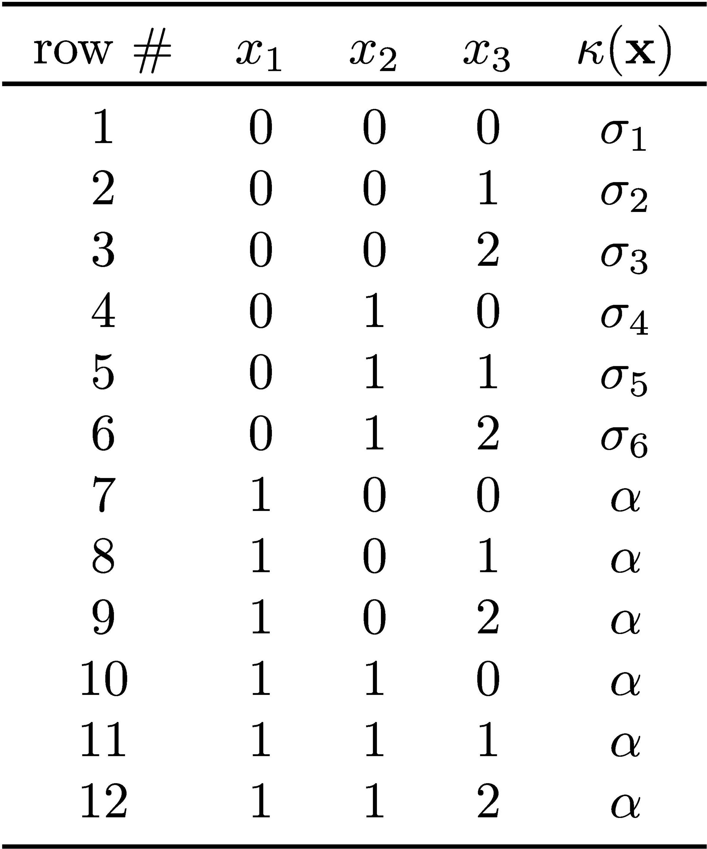
Parameterized example.  In the following sections, we consider a more general parameterized classifier, shown in Table 1, which encompasses the two classifiers shown in Figure 1. As clarified below, we impose that,

For simplicity, we also require that $\alpha ,{\sigma }_j\in Z,j=1,\dots ,6$. It is plain that the DT of Figure 1a is a concrete instantiation of the parameterized classifier shown in Table 1, by setting ${\sigma }_1={\sigma }_3={\sigma }_4={\sigma }_6=0$, ${\sigma }_2=4$, ${\sigma }_5=7$ and $\alpha =1$. For the parameterized example, the instance to be considered is $\left(\right(1,1,2),\alpha )$.

Table 1. 

Tabular representation of parameterized classifier, $\kappa$

Formal explanations.  We follow recent accounts of formal explainability.²⁴ In the context of XAI, abductive explanations (AXps) have been studied since 2018.^18,35 Similar to other heuristic approaches, for example, Anchors,³¹ abductive explanations are an example of explainability by feature selection, that is, a subset of features is selected as the explanation. AXps represent a rigorous example of explainability by feature selection, and can be viewed as the answer to a “Why (the prediction, given $\text{v}$)?” question. An AXp is defined as a subset-minimal (or irreducible) set of features $X\subseteq F$ such that the features in $X$ are sufficient for the prediction. This is to say that, if the features in $X$ are fixed to the values determined by $v$, then the prediction is guaranteed to be $c=\kappa \left(v\right)$. The sufficiency for the prediction can be stated formally:

For simplicity, we associate a predicate $\text{WAXp}$ (that is, weak AXp) with (2), such that $\text{WAXp}(X;E)$ holds if and only if (2) holds.

Observe that (2) is monotone on $X$,²⁴ and so the two conditions for a set $X\subseteq F$ to be an AXp (that is, sufficiency for prediction and subset-minimality), can be stated as follows:

A predicate $\text{AXp}:2^F\to \{0,1\}$ is associated with (3), such that $\text{AXp}(X;E)$ holds true if and only if (3) holds true.^d

An AXp can be interpreted as a logic rule of the form:

where $c=\kappa \left(v\right)$. It should be noted that informal XAI methods have also proposed the use of IF-THEN rules³¹ which, in the case of Anchors³¹ may or may not be sound.^16,18 In contrast, rules obtained from AXps are logically sound.

Moreover, contrastive explanations (CXps) represent a type of explanation that differs from AXps, in that CXps answer a “Why Not (some other prediction, given $\text{v}$)?” question.^17,28 Given a set $Y\subseteq F$, sufficiency for changing the prediction can be stated formally:

A CXp is a subset-minimal set of features which, if allowed to take a value other than the value determined by $v$, then the prediction can be changed by choosing suitable values to those features. As shown, and for simplicity, we associate a predicate $\text{WCXp}$ (that is, weak CXp) with (5), such that $\text{WCXp}(Y;E)$ holds if and only if (5) holds.

Similarly to the case of AXps, for CXps (5) is monotone on $Y$, and so the two conditions (sufficiency for changing the prediction and subset-minimality) can be stated formally as follows:

A predicate $\text{CXp}:2^F\to \{0,1\}$ is associated with (6), such that $\text{CXp}(Y;E)$ holds true if and only if (6) holds true.

Algorithms for computing AXps and CXps for different families of classifiers have been proposed in recent years (Marques-Silva²⁶ provides a recent account of the progress observed in computing formal explanations). These algorithms include the use of automated reasoners (for example, SAT, SMT or MILP solvers), or dedicated algorithms for families of classifiers for which computing one explanation is tractable.

Given an explanation problem $E$, the sets of AXps and CXps are represented by:

For example, $A\left(E\right)$ represents the set of all logic rules (of the type of rule (4)) that predict $c=\kappa \left(v\right)$, which are consistent with $v$, and which are irreducible (that is, no literal $x_i=v_i$ can be discarded).

Furthermore, it has been proved¹⁷ that (i) a set $X\subseteq F$ is an AXp if and only if it is a minimal hitting set (MHS) of the set of CXps; and (ii) a set $Y\subseteq F$ is a CXp if and only if it is an MHS of the set of AXps. This property is referred to as MHS duality, and can be traced back to the seminal work of R. Reiter²⁹ in model-based diagnosis. Moreover, MHS duality has been shown to be instrumental for the enumeration of AXps and CXps, but also for answering other explainability queries.²⁴ Formal explainability has made significant progress in recent years, covering a wide range of topics of research.^24,26

Feature (ir)relevancy.  Given (7) and (8), we can aggregate the features that occur in AXps and CXps:

Moreover, MHS duality between the sets of AXps and CXps allows one to prove that: $F_{A\left(E\right)}=F_{C\left(E\right)}$. Hence, we just refer to $F_{A\left(E\right)}$ as the set of features that are contained in some AXp (or CXp).

A feature $i\in F$ is relevant if it is contained in some AXp, that is, $i\in F_{A\left(E\right)}=F_{C\left(E\right)}$; otherwise it is irrelevant, that is, $i\notin F_{A\left(E\right)}$.^e A feature that occurs in all AXps is referred to as necessary. We will use the predicate $\mathrm{Relevant}\left(i\right)$ to denote that feature $i$ is relevant, and predicate $\mathrm{Irrelevant}\left(i\right)$ to denote that feature $i$ is irrelevant.

Relevant and irrelevant features provide a coarse-grained characterization of feature importance, in that irrelevant features play no role whatsoever in prediction sufficiency. In fact, the following logic statement is true iff $r\in F$ is an irrelevant feature:

The logic statement here clearly states that, if we fix the values of the features identified by any AXp then, no matter the value picked for feature $r$, the prediction is guaranteed to be $c=\kappa \left(v\right)$. The bottom line is that an irrelevant feature $r$ is absolutely unimportant for the prediction, and so there is no reason to include it in a logic rule consistent with the instance.

There are a few notable reasons for why irrelevant features are not considered in explanations. First, one can invoke Occam’s razor (a mainstay of ML⁴) and argue for simplest (that is, irreducible) explanations. Second, if irreducibility of explanations were not a requirement, then one could claim that a prediction using all the features would suffice, but that is never of interest. Third, the fact that irrelevant features can take any value in their domain without  impacting the value of the prediction shows how unimportant those features are.

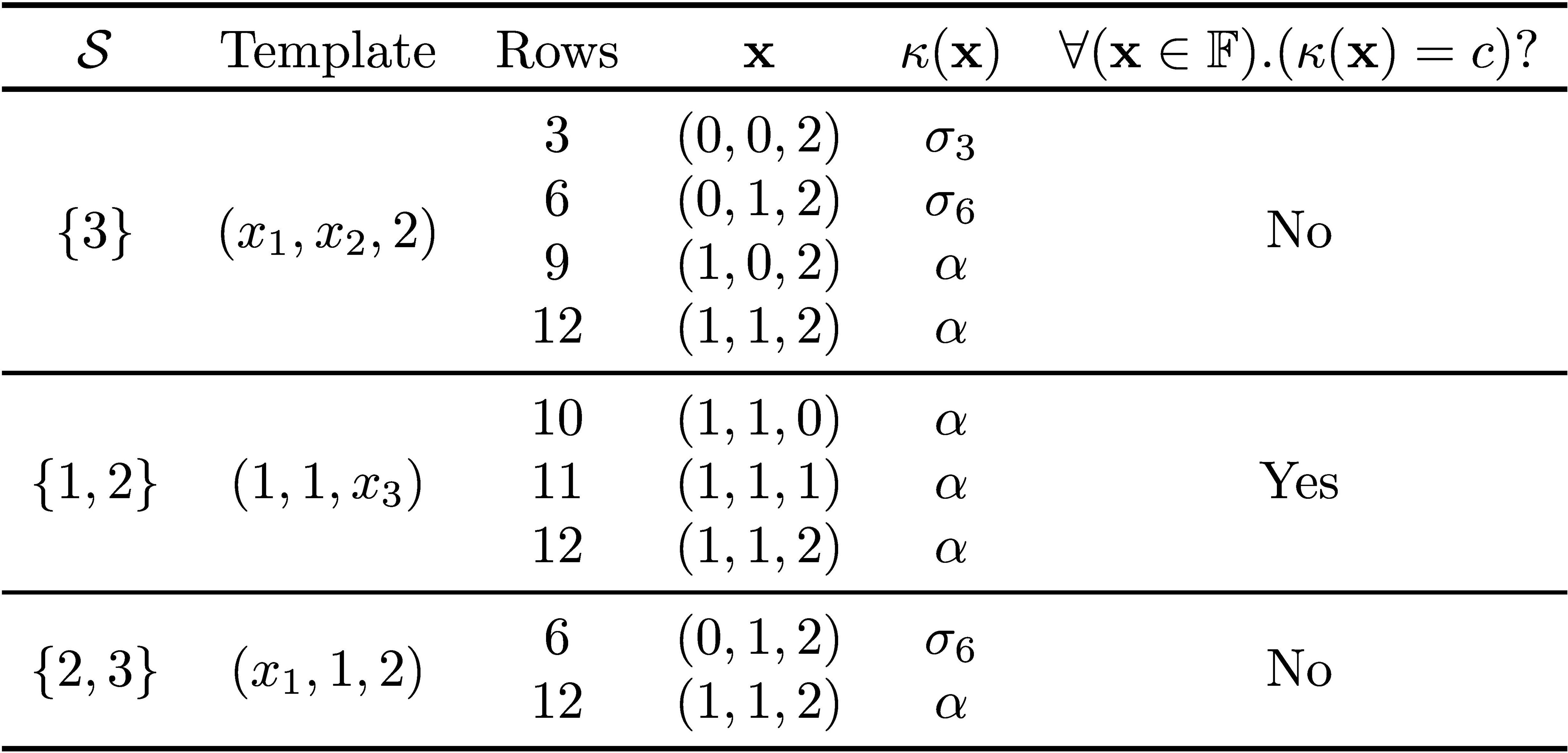
Explanations for running examples.  For both the classifiers of Figure 1 or the parameterized classifier of Table 1 (under the stated assumptions), it is simple to show that $A=\left\{\right\{1\left\}\right\}$ and that $C=\left\{\right\{1\left\}\right\}$. The computation of AXps/CXps is shown in Figure 2 for the parameterized classifier. More detail on how Figure 2 is obtained is given in Table 2. (Observe that computation of AXps/CXps shown holds as long as $\alpha$ differs from each of the ${\sigma }_i$, $i=1,\dots ,6$, that is, (1) holds.) Thus, for any of these classifiers, feature 1 is relevant (in fact it is necessary), and features 2 and 3 are irrelevant. These results agree with the analysis of the classifier (see Figure 1d) in terms of feature influence, in that feature 1 occurs in explanations, and features 2 and 3 do not. More importantly, there is no difference in terms of the computed explanations for either ${\kappa }_1$ or ${\kappa }_2$.

Table 2. 

Examples of how each set is analyzed when computing AXps. It is assumed that $\alpha \ne {\sigma }_i,i=1,\dots ,6$. For CXps, a similar approach is used.

As can be concluded, the computed abductive and contrastive explanations agree with the analysis shown in Figure 1d in terms of feature influence. Indeed, features 2 and 3, which have no influence in determining nor in changing the predicted class 1, are not included in the computed explanations, that is, they are irrelevant. In contrast, feature 1, which is solely responsible for the prediction, is included in the computed explanations, that is, it is relevant. Also unsurprisingly,^12,17,19 the existence of adversarial examples is tightly related with CXps, and so indirectly with AXps. These observations should be expected, since abductive explanations are based on logic-based abduction, and so have a precise logic formalization.

Adversarial examples.  Besides studying the relationship between SHAP scores and formal explanations, we also study their relationship with adversarial examples in ML models.¹¹

Hamming distance is a measure of distance between points in feature space. The Hamming distance is also referred to as the $l_0$ measure of distance, and it is defined as follows:

Given a point $v$ in feature space, an adversarial example (AE) is some other point $x$ in feature space that changes the prediction and such that the measure of distance $l_p$ between the two points is small enough:

(in our case, we consider solely $p=0$.)

The relationship between adversarial examples and explanations is well-known.^12,17,19

Similarly, it is straightforward to prove that,

Thus, irrelevant features are not included in subset- (or cardinality-) minimal adversarial examples.

Adversarial examples for running examples.  Given the previous discussion, and for $(v,c)=\left(\right(1,1,2),\alpha )$, it is plain that there exists an adversarial example with a $l_0$ distance of 1, which consists of changing the value of feature 1 from 1 to 0. This adversarial example is both subset-minimal and cardinality-minimal. As with formal explanations, the minimal adversarial example agrees with the analysis of the two classifiers included in Figure 1d.

Computing SHAP scores.  Let $\text{ϒ}:2^F\to 2^F$ be defined by,

that is, for a given set $S$ of features, and parameterized by the point $v$ in feature space, $\text{ϒ}(S;v)$ denotes all the points in feature space that have in common with $v$ the values of the features specified by $S$. Observe that $\text{ϒ}$ is also used (implicitly) for picking the set of rows we are interested in when computing explanations (see Figure 2).

Also, let $\varphi :2^F\to ℝ$ be defined by,

Thus, given a set $S$ of features, $\varphi (S;ℳ,v)$ represents the average value of the classifier over the points of feature space represented by $\text{ϒ}(S;v)$. The formulation presented in earlier work^1,2 allows for different input distributions when computing the average values. For the purposes of this article, it suffices to consider solely a uniform input distribution, and so the dependency on the input distribution is not accounted for.

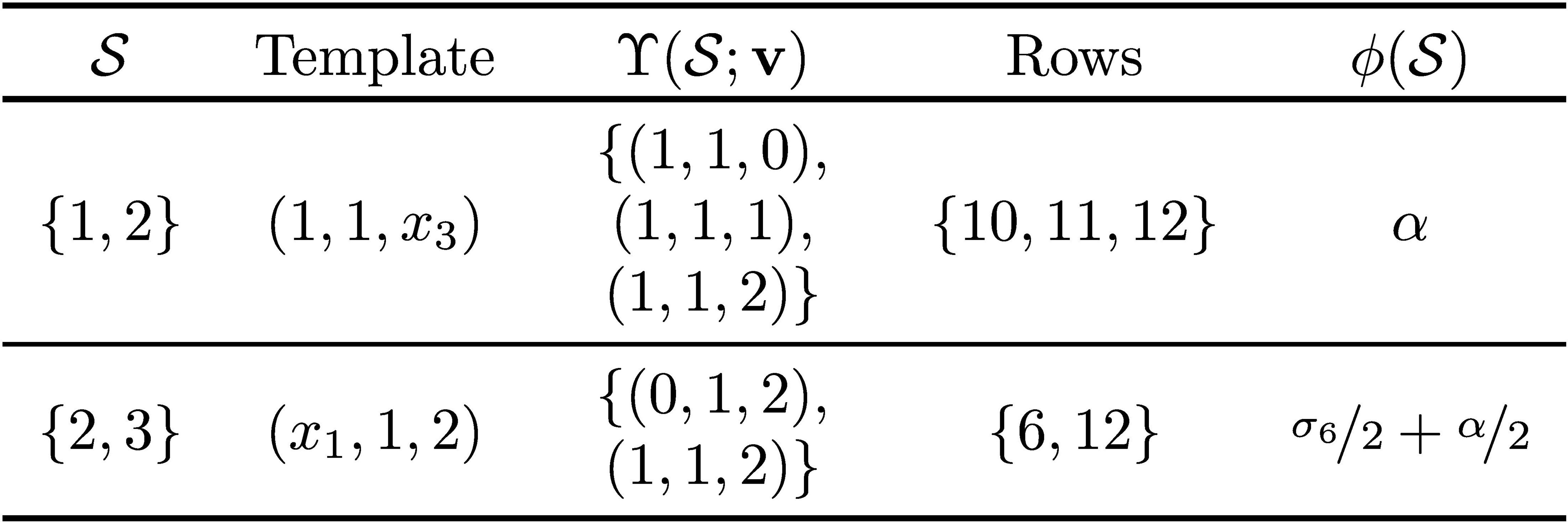
Table 3 illustrates how the average value is computed for two concrete sets of features. As an example, if $S=\left\{1\right\}$, then feature 1 is fixed to value 1 (as dictated by $v$). We then allow all possible assignments to features 2 and 3, thus obtaining,

To compute $\varphi \left(S\right)$, we sum up the values of the rows of the truth table indicated by $\text{ϒ}\left(S\right)$, and divide by the total number of points, which is 6 in this case.

Table 3. 

Computation of average values. Column ‘Rows’ shows the row numbers in Table 1 to consider when computing the average value.

To simplify the notation, the following definitions are used,

Finally, let $\text{Sc}:F\to ℝ$, that is, the SHAP score for feature $i$, be defined by,

Given an instance $(v,c)$, the SHAP score assigned to each feature measures the contribution of that feature with respect to the prediction. A positive/negative value indicates that the feature can contribute to changing the prediction, whereas a value of 0 indicates no contribution.³⁷

Misleading SHAP scores.  We now demonstrate that there is surprising flexibility in choosing the influence of each feature. Concretely, we want to show that SHAP scores can yield misleading information, and that this is easy to attain. To achieve this goal, we are going to create an evidently disturbing scenario. We are going to assign values to the parameters (that is, classes) of the classifier such that feature 1 will be deemed to have no importance on the prediction, and features 2 and 3 will be deemed to have some importance on the prediction. (Such choice of SHAP scores can only be considered misleading; as argued in Figure 1d, for either ${\kappa }_1$ or ${\kappa }_2$, predicting class 1 or predicting a class other than 1 depends exclusively on feature 1.) To obtain such a choice of SHAP scores, we must have (see Figure 3),

Clearly, there are arbitrarily many assignments to the values of $\alpha$ and ${\sigma }_j,j=1,\dots ,6$ such that constraints (18), (19), and (20) are satisfied. Indeed, we can express $\alpha$ in terms of the other parameters ${\sigma }_1\dots ,{\sigma }_6$, as follows:

In addition, we can identify values for ${\sigma }_j$, $j=1,\dots ,6$, such that the two remaining conditions (19) and (20) are satisfied. Moreover, we can reproduce the values in the DTs shown in Figure 1. Concretely, we pick $\alpha =1\wedge {\sigma }_1={\sigma }_3={\sigma }_4={\sigma }_6=0$ for both ${\kappa }_1$ and ${\kappa }_2$. Also, for ${\kappa }_1$, we choose ${\sigma }_2=4\wedge {\sigma }_5=7$. Finally, for ${\kappa }_2$, we choose ${\sigma }_2=2\wedge {\sigma }_5=3$. The resulting sets of SHAP scores, among others, are shown in Table 4.

Table 4. 

Computed SHAP scores for the instance $\left(\right(1,1,2),1)$, by setting $\alpha =1$ and ${\sigma }_1={\sigma }_3={\sigma }_4={\sigma }_6=0$, that is, DTs similar to those in Figures 1a and 1c, and where only the classes predicted in the terminal nodes 6 and 7 differ.

The results derived above confirm that, for the two running examples, in one case the SHAP scores give a rank of the features that must be misleading (that is, Figure 1a), whereas for the other case, the rank of the features is less problematic, in that the most important feature is attributed the highest relative importance (that is, Figure 1c). Evidently, it is still unsettling that for the second DT, the SHAP scores of irrelevant features are non-zero, denoting some importance to the prediction that other ways of analyzing the classifier do not reveal. As the two example DTs demonstrate, and even though their operation is exactly the same when $x_1=1$, the predictions made for points in feature space, that are essentially unrelated with the given instance, can have a critical impact on the relative order of feature importance. Whereas formal explanations and adversarial examples have a precise logic-based formalization, for the two example DTs (and also for the boolean classifiers discussed later in this article), there is no apparent logical justification for the relative feature importance obtained with SHAP scores.

We refer to the misleading information produced by SHAP scores as an example of an issue that can be formalized as follows:

The logic statement above may appear as rather specific, and so difficult to satisfy, because every feature must either be relevant and be assigned a zero SHAP score, or otherwise it must be irrelevant and be assigned a non-zero SHAP score. However, the example DT in Figure 1a shows that there are very simple classifiers with instances that satisfy the logic statement. Clearly, many other similarly simple examples could be devised. As we will clarify, Equation (22) is referred to as issue I8.

Revisiting the hypothetical scenario.  We consider again the instance $\left(\right(1,1,2),1)$, that is, an honors student from an urban household and majoring in sciences will enroll for 1 extra-curricular activity, for both DTs. Given the DTs or the TRs, formal explanations would deem the fact that she is an honors student as the answer to why the prediction is one extra-curricular activity. Also, to change the prediction, we would have to consider a non-honors student. Finally, to predict something other than 1 activity, while minimizing changes, then we would once again have to consider a non-honors student. Unsurprisingly, for the second DT (see Figure 1c), SHAP scores concur with assigning the most importance to the fact that the student is an honors student, even though SHAP scores assign some clearly unjustified importance to the other features. More unsettling, for the first DT (see Figure 1a), SHAP scores assign importance to the fact that the student is majoring in science, that she hails from an urban household, but entirely ignore the fact that she is an honors student. And the differences between the two DTs are only the number of extra-curricular activities of non-honors students who major in arts. The reason for this abrupt change in relative feature importance (that is, 1,3,2 to 3,2,1) is inscrutable.

Why do SHAP scores mislead?  We identified two reasons that justify why SHAP scores can provide misleading information: the contributions of all possible subsets of fixed features are considered; and class values are explicitly accounted for. For the examples studied in this article, these two reasons suffice to force SHAP scores to provide misleading information.