
In a forecasting exercise, Gordon Earle Moore, co-founder of Intel, plotted data on the number of components—transistors, resistors, and capacitors—in chips made from 1959 to 1965. He saw an approximate straight line on log paper (see Figure 1). Extrapolating the line, he speculated that the number of components would grow from 26 in 1965 to 216 in 1975, doubling every year. His 1965–1975 forecast came true. In 1975, with more data, he revised the estimate of the doubling period to two years. In those days, doubling components also doubled chip speed because the greater number of components could perform more powerful operations and smaller circuits allowed faster clock speeds. Later, Moore’s Intel colleague David House claimed the doubling time for speed should be taken as 18 months because of increasing clock speed, whereas Moore maintained that the doubling time for components was 24 months. But clock speed stabilized around 2000 because faster speeds caused more heat dissipation than chips could withstand. Since then, the faster speeds are achieved with multi-core chips at the same clock frequency.
Key Insights
- Exponential growth seems to be unique to computing and information technologies and their markets, stimulating continued economic, social, and political disruptions.
- Exponential growth occurs simultaneously at all levels of the computing ecosystem—chips, systems, adopting communities.
- Technology jumping sustains exponential growth as companies switch to new technologies when the current ones reach their points of diminishing return.
Moore’s Law is one of the most durable technology forecasts ever made.10,20,31,33 It is the emblem of the information age, the relentless march of the computer chip enabling a technical, economic, and social revolution never before experienced by humanity.
The standard explanation for Moore’s Law is that the law is not really a law at all, but only an empirical, self-fulfilling relationship driven by economic forces. This explanation is too weak, however, to explain why the law has worked for more than 50 years and why exponential growth works not only at the chip level but also at the system and market levels. Consider two prominent cases of systems evolution.
Supercomputers are complete systems, including massively parallel arrays of chips, interconnection networks, memory systems, caches, I/O systems, cooling systems, languages for expressing parallel computations, and compilers. Various groups have tracked these systems over the years. Figure 2 is a composite graph of data from these groups on the speeds of the fastest computers since 1940. The performance of these computers has grown exponentially. One of the tracking groups, TOP500 (https://www.top500.org/), has used a Linpack benchmark since 1993 to compare the fastest machines at each point in time for mathematical software, noting that the growth rate may be slowing because the market for such machines is slowing. The speeds of supercomputing systems depend on at least eight technologies besides the chips. How do we explain the exponential growth in this case?
Ray Kurzweil, futurist and author of The Singularity Is Near: When Humans Transcend Biology, formulated a set of predictions about information technology by constructing a graph of the computational speed growth over five generations of information technology (see Figure 3).25 He projected that this remarkable exponential doubling trend would continue for another 100 years, relying on jumps to new technologies every couple of decades. He also forecast a controversial claim—a “singularity” around 2040 when artificial intelligence will exceed human intelligence.25,32 The exponential growth in this case clearly does not depend on Moore’s Law at all. How do we explain the exponential growth in this case?
The three kinds of exponential growth, as noted—doubling of components, speeds, and technology adoptions—have all been lumped under the heading of Moore’s Law. Because the original Moore’s Law applies only to components on chips, not to systems or families of technologies, other phenomena must be at work. We will use the term “Moore’s Law” for the component-doubling rule Moore proposed and “exponential growth” for all the other performance measures that plot as straight lines on log paper. What drives the exponential growth effect? Can we continue to expect exponential growth in the computational power of our technologies?
Exponential growth depends on three levels of adoption in the computing ecosystem (see the table here). The chip level is the domain of Moore’s Law, as noted. However, the faster chips cannot realize their potential unless the host computer system supports the faster speeds and unless application workloads provide sufficient parallel computational work to keep the chips busy. And the faster systems cannot reach their potential without rapid adoption by the user community. The improvement process at all three levels must be exponential; otherwise, the system or community level would be a bottleneck, and we would not observe the effects often described as Moore’s Law.
With supporting mathematical models, we will show what enables exponential doubling at each level. Information technology may be unique in being able to sustain exponential growth at all three levels. We will conclude that Moore’s Law and exponential doubling have scientific bases. Moreover, the exponential doubling process is likely to continue across multiple technologies for decades to come.
Self-Fulfillment
The continuing achievement signified by Moore’s Law is critically important to the digital economy. Economist Richard G. Anderson said, “Numerous studies have traced the cause of the productivity acceleration to technological innovations in the production of semiconductors that sharply reduced the prices of such components and of the products that contain them (as well as expanding the capabilities of such products).”1 Robert Colwell, Director of DARPA’s Microsystems Technology Office, echoes the same conclusion, which is why DARPA has invested in overcoming technology bottlenecks in post-Moore’s-Law technologies.5 If and when Moore’s Law ends, that end’s impact on the economy will be profound.
It is no wonder then that the standard explanation of the law is economic; it became a self-fulfilling prophesy of all chip companies to push the technology to meet the expected exponential growth and sustain their markets. A self-fulfilling prophecy is a prediction that causes itself to become true. For most of the past 50-plus years of computing, designers have emphasized performance. Faster is better. To achieve greater speed, chip architects increased component density by adding more registers, higher-level functions, cache memory, and multiple cores to the same chip area and the same power dissipation. Moore’s Law became a design objective.
Designers optimize placement of components on highly constrained real estate, seeking to fill every square nanometer of area. Doubling component density—and therefore the number of components per nanometer of area—was not an outrageous objective because it requires only a reduction of 30% in both dimensions of 2D components. To achieve the next generation of Moore’s Law, designers halve the area of each component, which means reducing each dimension to sqrt(1/2) = 0.71 of its former value; we call this the “square root reduction rule.” Figure 4 shows that the die size of chips has consistently followed this rule over many generations. Wu et al.32 extended a quantum-limit argument offered by Nobel physicist Richard Feynman12 in 1985 to conclude that this downward scaling process could continue until device sizes approached the Compton wavelength of an electron, which will happen by approximately 2036.
Motivated by the promise of enormous economic payoffs, designers overcame many challenges to sustain this rule. Even so, we find self-fulfillment to be an unsatisfying explanation of the persistence of Moore’s Law. Why does the law not work for other technologies? What if systems had too many bottlenecks or workloads contained insufficient parallelism? What if people failed to adopt new technologies?
Moore’s Law at the Chip Level
What is special about information technologies that makes exponential growth a possibility? This possibility is not available for every technology. We might wish for automobiles that travel 1,600 miles on a gallon of gasoline—approximately six doublings (26) better than today’s most efficient automobiles—but wishing will not make it happen. There is no technology path leading to that level of automobile efficiency. What is different about chip technology?
The answer is that the basic performance measure of computing systems is computational steps per unit time (or energy). Twice as many components enable twice as many computational steps. And the regularity of components enables doubling them by scaling down size.
A chip is made of a very large number of simple basic components, mostly transistors and interconnecting wires. Doubling the number of components in a chip generation is a feasible goal, as in Figure 2, and a method called “Dennard scaling” (described in the following paragraphs) was invented to accomplish it. Few other technologies (such as automobiles) feature complex systems composed of large numbers of identical parts.
Component doubling every chip generation may be feasible but is not easy. The underlying silicon technology, CMOS, cannot support the continued component reductions. What are the problems? And what options are available to overcome them? We cover three main ones:
Path to the square root reduction rule. Dennard scaling, which defined a path to the square root reduction rule for nearly 30 years, why it came to an end, and what has been done to increase computational speed since then;
Clock trees and clock distribution. Why do we have clocks? What is the problem with clocked circuits? Could it be solved with an additional clock distribution layer on the chip? Or by replacing clocked circuits with fast asynchronous (unclocked) circuits?; and
Taxonomy. A taxonomy of issues needed to keep Moore’s Law at chip level going for more generations.
Dennard Scaling. In 1974, electrical engineer and inventor Robert Den-nard and his team at IBM proposed a method to scale down transistors while maintaining a constant power density.6 The power density is energy dissipated in a square unit of chip area. It is proportional to the switching speed and the number of transistors in a unit area. Greater power densities mean more heat to dissipate—and too much heat will burn up the chip. Dennard scaling says that power density stays constant as transistors get smaller so the power used is proportional to area.
Reducing the size of a subsystem and its components can allow for the clock interval to be shortened because the logic gates switch faster and the wires connecting them are shorter. As noted, however, there is a limit to this approach because the increased number of state switches produces more heat. Engineers were able to increase clock speeds from approximately 5MHz in 1981 (IBM PC) to approximately 2GHz in 2000, leveling off at approximately 3.5GHz since 2002 (Intel Pentium 4). The cost of heat-sink technology to support greater clock speeds is prohibitive.
Even when clock speeds were held constant, chip engineers started to discover in the 1990s that leakage and quantum-tunneling effects became significant at small dimensions and produced more heat than Dennard scaling predicted. Dennard scaling was no longer a reliable pathway to reducing component size.
Multicore architectures were the response to the demise of Dennard scaling. The first two-core chips had twice as many components as the previous one-core chips. They were organized as two CPUs running in parallel at the same limiting clock speed (approximately 3.5GHz). Two cores could achieve twice the one-core speed if the computational workload had multiple computational threads. However, doubling on-chip cores every generation has its own heat-dissipation problems that will limit how many cores can be usefully placed on a chip.11 Moreover, multicore architecture pushed some of the responsibility for speedup to multi-threaded programming and parallelizing compilers. Multicore parallelism is a fine strategy but draws programmers into parallel programming, something many were never trained to do.2
Metastability, clocks, and clock trees. Clocks became an integral feature of computer logic circuits in the 1940s because engineers could quickly and simply avoid a host of timing-dependent failures that result from metastable behavior in computer circuits. If the clock interval is too short, the flip-flops recording a subsystem’s state can be triggered before their inputs have settled down, risking internal oscillations that freeze circuits or cause other malfunctions (see Figure 5).7
Metastability is also an issue when asynchronous subsystems (no common clock) can sense unsettled signals in an attempt to synchronize with each other. Designers use special protocols (such as ready-acknowledge signaling) to minimize the risk of synchronization failure in those cases.7
Few other technologies (such as automobiles) feature complex systems composed of large numbers of identical parts.
A major design problem is transmitting signals from a clock to all the components that need clock signals. The wires that do this take space on the chip, and there is a propagation delay along each wire. The term “clock skew” refers to the difference between the path with shortest delay and the path with longest delay. To avoid metastability, engineers must choose the clock time long enough to overcome skew.
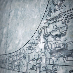
The ideal circuit to distribute clock signals is a balanced tree with the clock at its root and the components at its leaves. In a balanced tree, all paths are the same length, and there is no skew. Many designers considered the H-tree fractal, a mathematical model of a geometric tree structure that replicates at ever-finer dimensions with each generation (see Figure 6). However, the H-fractal is space-filling, meaning that as the dimension of the tree gets larger the area occupied by the wires eventually fills the chip, leaving little room for active components. This forces chip designers to use more ad hoc methods that depend on unbalanced trees restricted to a portion of the area (see Figure 7). The unbalanced trees have a much larger number of leaf nodes than needed, so the designer can choose leaf nodes nearest the components needing signals and minimize clock skew. Some designers propose to put a balanced H-tree on a new layer of the chip,27 but layering is controversial because putting other circuits (such as memory) on the new layer might benefit computing capacity more.
Due to these practical difficulties with clock-signal distribution, many designers have looked to asynchronous circuits. Two subsystems can exchange data by following a ready-acknowledge protocol. The sender signals that it has some data to send by setting a “ready” line to 1. On receipt of the signal, the receiver acknowledges by setting an “acknowledge” line to 1. When the sender sees the acknowledge, it deposits the data in a buffer and signals completion by returning “ready” to 0. Finally, the receiver takes the data from the buffer and sets “acknowledge” to 0. One unit of data can be transmitted at each cycle of this protocol.
Circuit designers have studied asynchronous signaling since the 1960s and developed reliable asynchronous circuits. Because these circuits are somewhat slower than clocked circuits, ready-acknowledge signaling is used only when there is no alternative (such as a CPU interacting with an I/O device).
Modern chips sometimes use asynchronous signaling (judiciously) to overcome clock distribution and skew problems. The chip is divided into modules, each with its own clock. Clocked circuits are used inside a module with asynchronous signaling between modules. For example, the module that displays a graphical image can be turned on just when a user wants to display the image and run at the clock speed necessary to render the image well; communication with the display module can be asynchronous.
Designing an all-asynchronous computer has been a holy grail among circuit designers for years. Intel is said to have demonstrated an asynchronous circuit for the fetch-execute control of a CPU but has not yet succeeded at creating an arithmetic-logic unit (ALU). The main research problem is finding a way for the ALU to report when it is done with an operation, given that the time of the operation can vary significantly depending on the inputs. Computer graphics pioneer Ivan Sutherland has long advocated for all-asynchronous circuits and demonstrated asynchronous pipeline chips.30 Perhaps the most complete design of a computer that has no clocks is the dataflow architecture proposed by computer scientist Jack Dennis.9 It did not inspire sufficient commercial interest because its circuits ran slower than conventional clocked circuits; the machine got its throughput from massive data parallelism, which was not common at the time. Because the number of data-intensive applications continues to grow, the massively parallel dataflow architecture may yet find acceptance.
Potential technology directions. Many engineers have been studying how to enable the continued growth of Moore’s Law, given that the existing CMOS technology cannot be pushed much further; for more on the intensive research in this area, see the sidebar “Technology Jumping in Pursuit of Moore’s Law.”
Exponential Growth at the System Level
Users of computation are hungry for performance, measured as calculations per second or (more recently) calculations per watt-hour. But it does little good to embed faster chips in systems that are limited by other bottlenecks (such as communication bandwidth and cooling systems).
Bottlenecks are the main barrier to performance in systems. Engineers spend a lot of time identifying bottlenecks and speeding them up. Each generation of system improvement is more challenging because engineers must search multiple new technologies to resolve all bottlenecks.
Colwell5 discussed bottlenecks generated by “neighboring technologies,” or technologies from other fields on which microchips depend. Wu et al.33 gave a nice example with ubiquitous modern analog-digital converters (ADC). ADCs sample a continuous input signal at twice its highest frequency, producing a series of digital snapshots; according to the Nyquist sampling theorem, no information is lost at this sampling rate because the continuous signal can be regenerated from the samples. As logic circuits get faster, the ADC sampling rate is itself eventually a bottleneck. Engineers are searching for new sampling methods with higher rates.
The memory system is another potential bottleneck. Caches are a critical driver of performance; modern chips rely extensively on caches to position needed data near the processor, and poorly positioned data slows the cache and, in turn, the processor. Considerable research effort has gone into measuring locality of workloads and designing the caches for optimal performance with those workloads. Cache designers are under constant pressure to produce memory improvements matching CPU improvements.
Despite these challenges, computer engineers have been very successful over the years at producing complete systems with performance that has grown exponentially. Koomey22,23 gathered data for a large number of different computers from 1946 to 2009 and found exponential growth in two measures: computation speeds per computer and computations per kilowatt-hour (kwh); see Figure 8 for his graph of computations per kwh. The doubling times were about the same—1.57 years—in both graphs. The improvements relative to energy consumption, summarized as Koomey’s Law,10 have assumed great importance in an energy-constrained world, from large data centers with fixed power draw to mobile devices with fixed battery life. This trend could continue for at least another several decades.
Even when systems are designed so no bottlenecks stand in the way of performance, it is possible that the workloads presented to those systems are not sufficient to use all the available computing power. In 1967, Gene Amdahl, a mainframe computer designer at IBM, investigated whether it would be better to get faster speed through a faster CPU or through several slower parallel CPUs. Based on his experience designing instruction-lookahead CPUs, he realized that substantial parts of code must be executed sequentially in the given compiled sequence; only some of the instructions could be speeded up by parallel execution. He derived a formula that became known as Amdahl’s Law to express the speedup potential from a set of n processors (cores) working on a program. Amdahl’s idea—expressing the parallelizable part as a set of parallel instruction streams—was known in his time as “control parallelism.” Suppose the time of the job using 1 stream is T(1) = a+b, where a is the time for the serial part, and b is the time for the parallelizable part. The serial fraction is p = a/(a+b), and parallelizable fraction is 1-p. The time to execute on n streams is T(n) = a + b/n because only the control-parallel portion of the algorithm can benefit from n processors. Amdahl’s Law says the speedup is

For example, an application 10% serial would run at most 10 times faster than its single-stream time, even with a large number of parallel processing cores. That is, even if a small part of the overall computation is serial, it is impossible to achieve much multicore speedup with control parallelism.18
Amdahl’s Law would seem to limit the speedup to considerably less than the number of cores, because it assumes parallelism comes from remodeling a serial algorithm into a parallel algorithm. However, Amdahl’s Law overlooks parallelism inherent in data. Data-parallel workloads are now common in data-intensive applications (such as MapReduce operations on the Web). In a data-intensive problem, the data space can be partitioned into many small subsets, each of which can be processed by its own thread. The finer the grain of the partition, the larger the number of threads. The same algorithm runs in each thread on the data subset belonging to that thread. Computer scientist John Gustafson observed that large data-intensive problems could always be partitioned into as many grains as could be supported by cores in the processors when there is sufficient data parallelism.16 In this case, the computational work completed on one core is W(1) = a+b, as outlined earlier. With n cores, it jumps to W(n) = a + bn because each of the n cores is performing the same operation on its thread’s (different) data items. Gustafson’s Law says the speedup is linear in n

That is, for data-intensive applications with small serial fraction p, adding cores increases the computational work in direct proportion to the number of cores.
Rather than parallelizing the algorithm, data-parallel programming parallelizes the data. Gustafson’s Law models data-parallel computing, where the speedup scales with the size of the data, not the number of control-parallel paths specified in the algorithm.
Parallelizing data instead of algorithms was a paradigm shift that began in the 1980s.8 Today, it exploits multicore systems even when algorithms cannot be parallelized. It extends to heterogeneous data parallelism for common applications on the Internet (such as querying databases, serving email, and executing graphics-intensive applications, as in games). Peer-to-peer computing is a form of loosely coupled data parallelism, and cloud computing with multicore servers is a form of tightly coupled data parallelism.
Data parallelism and its variants is why multicore systems can continue to double output without increasing clock frequency. At the system level, as long as the applications contain many parallel tasks, there is always work available for the new cores in next-generation systems. This paradigm is especially useful for processing big data now being routinely provided by users of products from companies like Google, Facebook, Twitter, and LinkedIn.
Technology Diffusion at the Community Level
Moore spoke of a second law, also known as Rock’s Law, which is less well known than Moore’s own component-doubling law. The second law says that the cost of the fabrication facility for new chips doubles approximately every four years. This is due to the greater precision and ever-smaller size of lithography. An important implication is that the market for a new generation of chips at the same price must be at least double the market for the current generation, just to pay for the new fabrication facility. That is, Moore and Rock recognized that the markets had to expand exponentially to support the continuation of the basic Moore’s Law. Without exponential expansion of adoption at the community level, Moore’s Law at the chip level would be unsustainable.
Many business strategists believe in the S-curve model whereby the number of people using a technology initially grows exponentially to an inflection point and then flattens out (see Figure 9). The flattening out is caused by the saturation of the market—no more new adopters. Businesses try to time their entry into new technologies whose new S-curves are in their exponential growth stage when the older technology starts to flatten, or “technology jumping.” Businesses ride a series of S-waves and experience continuous exponential growth as they hop from one wave to the next.
Technology jumping is an integral, recurrent theme in computing. We noted earlier that Kurzweil explained exponential growth in the power of information technology by five massive switches to new technology that made older ones obsolete.25 He assumed that the process of technology jumping will continue well into the 21st century. Steve Jobs of Apple spoke frequently about his strategy of timing his jump to the next technology with the inflection point of the S-curve for the current technology. Andy Grove of Intel took the emergence of a new technology that did a job 10 times better than the current technology as a sign of an inflection point and built his company’s strategy around well-timed jumps.15
Whether or not a new technology is adopted depends on whether people use it instead of something else to accomplish something they care about.13 Innovators play an important role in this process by making products and services that influence community members to commit to adopt the new technology into their practice.
A simple argument shows why initial growth of adoption is exponential. Suppose n(t) is the number of members of a population who have adopted a technology as of time t. Each adopter demonstrates the value of the new technology to the rest of the population. Let a be the rate at which one adopter influences a non-adopter to adopt. In a small time interval h, the probability that a new adopter comes on board is ah. At time t+h, there are thus ahn(t) new adopters, giving n(t+h)−n(t) = ahn(t). Rearranging this equation and letting h go to 0 yields the differential equation

The solution to this equation is n(t) = eat. The size of the adopting population increases exponentially and the mean time between adoptions is 1/a. We can conclude from this simple equation that exponential growth happens when the rate of change also increases with current state.
This model is also too simple because it does not account for diminishing returns due to market saturation or technology reaching a limit where growth stops, when, for example, everyone in the population has adopted the technology. We can extend the model to account for the diminishing population of non-adopters. As before, let n(t) denote the number of members in a population of size N who have adopted a technology. The change in the number of adopters from time t to time t+h would then be proportional to two quantities: the number who have already adopted, as in equation 3, and the fraction who have not yet adopted. This gives the differential equation

which is called the “logistics equation” in the literature; its solution is

This function grows exponentially to its inflection point. Initially, when t=0, there is only one adopter, n(0) = 1, and after a long period of time there are N adopters.
Reality is more complicated because individuals have their own adoption time constants. Sociologist Everett Rogers discovered in 1962 that individuals fall into five groups according to the time they take to commit to an adoption—innovator, early adopter, early majority, late majority, and laggard.28 The histogram of adoption times follows a Bell curve. The five categories correspond to five zones of standard deviations. For example, innovators are 2.5% of the population, with adoption times at least two standard deviations below the mean; early adopters are 13.5% and are one to two standard deviations below the mean; early majority are 34% and zero to one standard deviations below the mean. In 1969, professor of marketing Frank Bass modified the Rogers diffusion model by quantifying the impact of early-adopter and word-of-mouth (all other) followers, inserting parameters p (early adoption rate), q (word-of-mouth follower rate), and N into the simple logistics curve.3,4 Ashish Kumar and others have since validated Bass’s extensions for real products by finding parameters p, q, and N for a number of technology products.14,24 Setting a=p+q and r=q/p, the Bass model then gives

Bass’s equation is still a logistics model that more accurately forecasts sales and also reaches an inflection point where the exponential growth begins to slow as diminishing returns set in. Figure 10 depicts four different technology adoptions since 1980. Bass’s model can be solved to find the inflection-point value of at, helping fit the model to data.
Data parallelism and its variants is why multicore systems can continue to double output without increasing clock frequency.
No matter what, the initial growth up to the inflection point is exponential. Historically, information technologists have jumped from one technology to another when an incumbent technology nears its inflection point. After each jump, they are on a new curve growing exponentially toward a new inflection point. Moore’s Law, and others like it, are intrinsically exponential because their rate of change is proportional to their current state.
Conclusion
The original 1965 Moore’s Law was an empirical observation that component density on a computer chip doubled every two years. Similar doubling rates have been observed in chip speeds, computer speeds, and computations per unit of energy. However, the durability of these technology forecasts suggests deeper phenomena.
We have argued that exponential growth would not have succeeded without sustained exponential growth at three levels of the computing ecosystem—chip, system, and adopting community. Growth (progress) feeds on itself up to the inflection point. Diminishing returns then set in, signaling the need to jump to another technology, system design, or class of application or community.
At the chip level, there are strong economic motivations for chip companies and their engineers to feed on previous improvements, building faster chips that grow exponentially up to the inflection point. The first significant technology path for exponential chip growth appeared in the form of Dennard scaling, which showed how to reduce component dimension without increasing power density. Dennard scaling reached an inflection point in the 1990s due to heat-dissipation problems that limited clock speed to approximately 3.5Ghz. Engineers responded with a technology jump to multicore chips, which gave speedup through parallelism. This jump has been enormously effective. Cloud platforms and supercomputers achieve high computation rates through massive parallelism among many chips.
A major technology barrier to chip growth has been the distribution of clock signals to all components on a chip. The theoretically most efficient distribution mechanism is the space-filling fractal H-tree that reaches diminishing returns when the tree itself starts to consume most of the physical space on the chip. Engineers are experimenting with hybrids that feature subsystems (such as cores) with their own clocks interacting via asynchronous signaling. Some engineers have been exploring the design of all-asynchronous circuits (no clocks), but these systems cannot yet compete in speed with clocked systems.
Engineers have been systematically examining the barriers that prevent the continuation of Moore’s Law for CMOS technologies. As alternatives mature, it will be feasible to jump to the new technologies and continue the exponential growth. Although there is controversy about how successful some of the alternatives may be, there is considerable optimism that some will work out and exponential growth can continue with new base technologies.
When chips and other components are assembled into complete computer systems, engineers have located and relieved technology bottlenecks that would prevent the systems from scaling up in speed as fast as their component chips scale. Koomey’s Laws document exponential growth of computations per computer and per unit of energy from 1946 to 2009. Koomey’s Law for computations per unit of energy is especially important throughout an energy-constrained industry. Additionally, the technology jump from algorithm parallelism to data parallelism further assures us we can grow systems performance as long as the workloads have sufficient parallelism, which has turned out to be the case for cloud and supercomputing systems.
Finally, we demonstrated that simple assumptions about adoption process lead to the S-curve model in which adoptions grow exponentially until an inflection point and then slow down because of market saturation. Business leaders use the S-curve model to guide them in jumping to new technologies when the older ones start to encounter their limits. Exponential growth in sales through ever-expanding applications and communities provides the financial stimulus to advance the chip-and system-level technologies (Rock’s Law). It is a complete cycle.
These analyses show that the conditions exist at all three levels of the computing ecosystem to sustain exponential growth. They support the optimism of many engineers that many additional years of exponential growth are likely. Moore’s Law was sustained for five decades. Exponential growth is likely to be sustained for many more.
Acknowledgments
We are grateful to Douglas Fouts and Ted Huffmire, both of the Naval Postgraduate School, Monterey, CA, for conversations and insights as we worked on this article.
Figures
 Figure 1. Moore’s original prediction graph showed component count followed a straight line when plotted on log paper.26
 Figure 2. Speeds of the fastest computers from 1940 show an exponential rise in speed. From 1965 to 2015, the growth was a factor of 12 orders of 10 over 50 years, or a doubling approximately every 1.3 years.
 Figure 3. Kurzweil’s graph of speed of information technologies since 1900 spans five families of technologies. From 1900 to 2000, the growth was 14 orders of 10 over 100 years, or a doubling approximately every 1.3 years.
 Figure 4. Logarithm of actual versus predicted feature size since 1970 matches a straight line with regression coefficient R2 = 0.97. Future sizes are predicted by dividing the previous size by sqrt(2); see the open triangles and dotted line. Future sizes two generations into the future are close to half the current sizes; see the square dots.
 Figure 5. Computer subsystems are organized as stateless logic circuits (AND, OR, NOT gates without feedback loops) driving flip-flops that record the subsystem’s state. Clock pulses trigger the flip-flops (X1,…,Xk) to assume the states generated by the logic outputs. Too short a clock interval risks a metastable state because the logic outputs driving the flip-flops may not have settled since the last clock pulse.
 Figure 6. Four iterations of the space-filling H-tree fractal show how to quadruple the number of terminal nodes by halving the size of each “H.” Each iteration appends a half-size “H” to the terminal nodes of the previous “H.” A clock signal is injected at the center and arrives at all the terminal nodes simultaneously because the H-tree is balanced; see http://www.tamurajones.net/FractalGenealogy.xhtml
 Figure 7. Design of an actual chip has approximately half its area devoted to the clock tree (dense lines) and half to its actual components (colored boxes). Image courtesy of Sung Kyu Lim at The Georgia Institute of Technology.27
 Figure 8. Koomey’s Law graph illustrates the continuing success of designing systems that produce more computation for the same power consumption. Careful power management over the past decade has enabled the explosion of mobile devices that depend critically on technologies that minimize power use.
 Figure 9. The logistics function—the mathematical model for growth of a population (such as adopters of a technology)—plots as an S-curve (black) over time. Initially, the curve follows an exponential (red) curve, but after an inflection point (here at time 6) it flattens out because of market saturation.
 Figure 10. Four different technology-adoption histories illustrate how versatile the Bass model is for accurately representing and forecasting technology adoptions. Data gleaned from Gentry,14 Jones,21 and Kumar.24
 Figure. Watch the authors discuss their work in this exclusive Communications video. http://cacm.acm.org/videos/exponential-laws-of-computing-growth


Join the Discussion (0)
Become a Member or Sign In to Post a Comment