We describe a new vector-based primitive for creating smooth-shaded images, called the diffusion curve. A diffusion curve partitions the space through which it is drawn, defining different colors on either side. These colors may vary smoothly along the curve. In addition, the sharpness of the color transition from one side of the curve to the other can be controlled. Given a set of diffusion curves, the final image is constructed by solving a Poisson equation whose constraints are specified by the set of gradients across all diffusion curves. Like all vector-based primitives, diffusion curves conveniently support a variety of operations, including geometry-based editing, keyframe animation, and ready stylization. Moreover, their representation is compact and inherently resolution independent. We describe a GPU-based implementation for rendering images defined by a set of diffusion curves in real time. We then demonstrate an interactive drawing system for allowing artists to create artworks using diffusion curves, either by drawing the curves in a freehand style, or by tracing existing imagery. Furthermore, we describe a completely automatic conversion process for taking an image and turning it into a set of diffusion curves that closely approximate the original image content.
1. Introduction
Vector graphics, in which images are defined with geometric primitives such as lines, curves, and polygons, dates back to the earliest days of computer graphics. Early cathode-ray tubes, starting with the Whirlwind-I in 1950, were all vector displays, while the seminal Sketchpad system24 allowed users to manipulate geometric shapes in the first computer-aided design tool. Raster graphics provides an alternative representation for describing images via a grid of pixels rather than geometry. Raster graphics arose with the advent of the framebuffer in the 1970s and is now commonly used for storing, displaying, and editing images. However, while raster graphics offers some advantages over vector graphics—primarily, a more direct mapping between the hardware devices used for acquisition and display of images, and their internal representation—vector graphics continues to provide certain benefits as well. Most notably, vector graphics offers a more compact representation, geometric editability, and resolution independence (allowing scaling of images while retaining sharp edges, see Figure 2). Vector-based images are also more easily animated through keyframe animation of their underlying geometric primitives. For all of these reasons, vector-based drawing tools, such as Adobe Illustrator©, CorelDraw©, and Inkscape©, continue to enjoy great popularity, as do standardized vector representations such as Flash and SVG.
However, for all of their benefits, vector-based drawing tools offer only limited support for representing complex color variations. For example, the shading of the turtle in Figure 2 is only depicted with uniform color regions, and most existing vector formats support only linear or radial gradients. A more sophisticated vector-based tool for handling complex gradients is the gradient mesh. A gradient mesh is a lattice with colors at each vertex that are interpolated across the mesh. While more powerful than simple gradients (or “ramps”), gradient meshes still suffer from some limitations. A significant one is that the topological constraints imposed by the mesh lattice give rise to an overcomplete representation that becomes increasingly inefficient and difficult to create and manipulate due to the high number of control points. Although automatic generation techniques15, 23, 25 have been recently proposed, they do not address the process of subsequent gradient-mesh manipulation, nor do they facilitate free-hand creation of gradient meshes from scratch.
In this paper we propose an alternative vector-graphics primitive, called the diffusion curve. A diffusion curve is a curve that diffuses colors on both sides of the space that it divides. The motivations behind such a representation are twofold:
First, this representation supports traditional free-hand drawing techniques where artists begin by sketching shapes, then adding color later. Similarly, users of our tool first lay down drawing curves corresponding to color boundaries. In contrast with traditional vector graphics, the color boundaries do not need to form closed geometric shapes and may even intersect. For example, the cloth in Figure 1 is created with open curves that have different colors on each side. The diffusion process then creates smooth gradients between nearby curves. Closed curves can be used to define regions of constant colors, such as the eyebrows in Figure 1. By specifying blur values along a curve, artists can also create smooth color transitions across the curve boundaries, like on the cheek of the character in Figure 1.
Second, most color variations in an image can be assumed to be caused by edges (material and depth discontinuities, texture edges, shadow borders, etc.).14, 18 Even subtle shading effects can be modeled as though caused by one or more edges, and it has been demonstrated that edges can be used to encode and edit images.6, 8, 9 In this work, we rely on vision algorithms, such as edge detection, to convert an image into our diffusion curves representation fully automatically.
The main contribution of this paper is therefore the definition of diffusion curves as a fundamental vector primitive, along with two types of tools: (1) A prototype allowing manual creation and editing of diffusion curves. Thanks to an efficient GPU implementation, the artist benefits from instant visual feedback despite the heavy computational demands of a global color diffusion. (2) A fully automatic conversion from a bitmap image based on scale-space analysis. The resulting diffusion curves faithfully represent the original image and can then be edited manually.
2. Previous Work
We review here existing techniques to create complex color gradients with modern vector graphics tools. We also mention methods to convert photographs in vector images with these techniques.
For a long time, vector graphics has been limited to primitives (paths, polygons) filled with uniform color or linear and radial gradients. Although skillful artists can create rich vector art with these simple tools, the resulting images often present flat or limited shading. The SVG format and modern drawing tools (Adobe Illustrator©, Corel CorelDraw©, Inkscape©) allow the creation of smooth color variations by blurring the vector primitives after rasterization. Nevertheless, artists often need to combine multiple primitives to create complex shading effects. Gradient meshes have been introduced in Adobe Illustrator© and Corel CorelDraw© to address these limitations. This tool produces smooth color variations over the faces of a quad mesh by interpolating the color values stored at its vertices. However, creating a mesh requires much skill and patience, because the artist needs to anticipate the mesh resolution and orientation necessary to embed the desired image content. This is why most artists rely on an example bitmap to drive the design of realistic gradient meshes. In addition, because the mesh resolution needs to be high enough to capture the finest image features, it is often unnecessarily high for nearby smoothly varying regions that could be represented with much fewer information. This constraint makes gradient meshes tedious to manipulate.
An alternative to manual creation is to convert an existing bitmap image into a vector representation. Commercial tools such as Adobe Live Trace© convert bitmap images into vector graphics by segmenting the image into regions of constant color and fitting polygons onto these regions. The resulting images often have a cartoon style similar to Figure 2 due to color quantization. The ArDeco system of Lecot and Levy16 produces smoother images by approximating color variations inside regions with linear or radial gradients. Similarly, several systems have been proposed to approximate a bitmap image with a collection of gradient meshes, either with user assistance23 or automatically.25
The new representation described in this paper offers the same level of visual complexity as that reached by gradient meshes, but has two main advantages: it is sparse, and corresponds to meaningful image features. Diffusion curves do not impose connectivity and do not require superfluous subdivision, which facilitates the manipulation of color gradients. Moreover, our representation naturally lends itself to automatic extraction from a bitmap image: we use an edge detector to locate curves and image analysis algorithms to estimate curve attributes (color and blur).
In other words, compared to regions used in classic vector representations, or patches used in gradient meshes, our approach is motivated by the fact that most of the color variation in an image is caused by or can be modeled with edges; and that (possibly open) regions or patches are implicitly defined in between. Such a sparse image representation is strongly motivated by the work of Elder8, who demonstrated that edges can faithfully encode images. Elder and Goldberg9 also suggested the possibility of using edges to manipulate images with basic operations (edge delete, copy, and paste). However, we believe the full potential of this approach has yet to be attained. For this reason, our conversion algorithm starts from the same premises as Elder’s system. By vectorizing edges and their attributes, we extend manipulation capabilities to include shape, color, and blur operations and we support resolution independence and keyframe animation.
3. Diffusion Curves
In this section we introduce the basic primitive of our representation, called a diffusion curve, and describe how to efficiently render an image from such primitives. Creation and manipulation of diffusion curves are discussed in subsequent sections.
The basic element of a diffusion curve is a geometric curve defined as a cubic Bézier spline (Figure 3(a)) specified by a set of control points P. The geometry is augmented with additional attributes: two sets of color control points Cl and Cr (Figure 3(b)), corresponding to color constraints on the right and left half space of the curve; and a set of blur control points (Σ) that defines the smoothness of the transition between the two halves (Figure 3(c)). As a result, the curves diffuse color on each side with a soft transition across the curve given by its blur (Figure 3(d)).
Color and blur attributes can vary along a curve to create rich color transitions. This variation is guided by an interpolation between the attribute control points in attribute space. In practice, we use linear interpolation and consider colors in RGB space throughout the rendering process, because they map more easily onto an efficient GPU implementation and proved to be sufficient for the artists using our system. Control points for geometry and attributes are stored independently, since they are generally uncorrelated. This leads to four independent arrays in which the control points (geometry and attribute values) are stored together with their respective parametric position t along the curve:

The diffusion curves structure encodes data similar to Elder’s edge-based representation.8 However, the vectorial nature of a diffusion curve expands the capabilities of Elder’s discrete edges by allowing precise control over both shapes—via manipulation of control points and tangents—and appearance attributes—via color and blur control points (small circles on the Figures). This fine-level control, along with our real time rendering procedure, facilitates the drawing and editing of smooth-shaded images.
 3.2. Rendering smooth gradients from diffusion curves
Three main steps are involved in our rendering model (see Figure 4): (1) rasterize a color sources image, where color constraints are represented as colored curves on both sides of each Bézier spline, and the rest of the pixels are uncolored; (2) diffuse the color sources similarly to heat diffusion—an iterative process that spreads the colors over the image; we implement the diffusion on the GPU to maintain real time performance; and (3) reblur the resulting image with a spatially varying blur guided by the blur attributes.
Color sources. Using the interpolated color values, the first step renders the left and right color sources cl(t), cr(t) for every pixel along the curves. An alpha mask is computed along with the rendering to indicate the exact location of color sources versus undefined areas.
For perfectly sharp curves, these color sources are theoretically infinitely close to each other. However, rasterizing points separated by too small a distance on a discrete pixel grid leads to overlapping pixels. In our case, this means that several color sources are drawn at the same location, creating visual artifacts after the diffusion. Our solution is to distance the color sources from the curve slightly, and to add a color gradient constraint directly on the curve. The gradient maintains the sharp color transition, while the colors, placed at a small distance d in the direction normal to the curve, remain separate.
More precisely, the gradient constraint is expressed as a gradient field w which is zero everywhere except on the curve, where it is equal to the color derivative across the curve. We decompose the gradient field in a gradient along the x direction wx and a gradient along the y direction wy. For each pixel on the curve, we compute the color derivative across the curve from the curve normal N and the left (cl) and right (cr) colors as follow (we omit the t parameter for clarity): wx,y = (cl − cr)Nx,y.
We rasterize the color and gradient constraints in 3 RGB images: an image C containing colored pixels on each side of the curves, and two images Wx, Wy containing the gradient field components. In practice, the gradient field is rasterized along the curves using lines of one pixel width. Color sources are rasterized using triangle strips of width 2d using a pixel shader that only draws pixels that are at a distance d from the curve (Figure 4(1)). In our implementation d is set at 3 pixels. Pixel overlap can still occur along a curve in regions of high curvature (where the triangle strip overlaps itself) or when two curves are too close to each other (as with thin structures or intersections). A simple stencil test allows us to discard overlapping color sources before they are drawn, which implies that solely the gradient field w dictates the color transitions in these areas. An example of such case can be seen in Figure 1, where the eyebrows are accurately rendered despite their thin geometry.
Diffusion. Given the color sources and gradient fields computed in the previous step, we next compute the color image I resulting from the steady state diffusion of the color sources subject to the gradient constraints (Figure 4(2)). Similar to previous methods,6, 8 we express this diffusion as the solution to a Poisson equation, where the color sources impose local constraints:

where Δ and div are the Laplace and divergence operators.
Computing the Poisson solution requires solving a large sparse linear system, which can be very time consuming if implemented naively. To offer interactive feedback to the artist, we solve the equation with a GPU implementation of the multigrid algorithm.4, 19 The idea behind multigrid methods is to use a coarse version of the domain to efficiently solve for the low frequency components of the solution, and a fine version of the domain to refine the high frequency components. We use Jacobi relaxations to solve for each level of the multigrid, and limit the number of relaxation iterations to achieve real time performance. Typically, for a 512×512 image we use 5i Jacobi iterations per multigrid level, with i the level number from fine to coarse. This number of iterations can then be increased when high quality is required. All the images in this paper have been rendered using an Nvidia GeForce 8800, providing real time performance on a 512×512 grid with a reasonable number of curves (several thousands). Jeschke et al.11 describe a GPU solver dedicated to diffusion curves with improved performance.
Reblurring. The last step of our rendering pipeline takes as input the color image containing sharp edges, produced by the color diffusion, and reblurs it according to blur values stored along each curve. However, because the blur values are defined only along curves, we lack blur values for off-curve pixels. A simple solution, proposed by Elder,8 diffuses the blur values over the image similarly to the color diffusion described previously. We adopt the same strategy and use our multi-grid implementation to create a blur map B from the blur values. The only difference to the color diffusion process is that blur values are located exactly on the curve so we do not require any gradient constraints. This leads to the following equation:

Given the resulting blur map B, we apply a spatially varying blur on the color image (Figure 4(3)), where the size of the blur kernel at each pixel is defined by the required amount of blur for this pixel. Despite a spatially varying blur routine implemented on the GPU,1 this step is still computationally expensive for large blur kernels (around one second per frame in our implementation), so we bypass it during curve drawing and manipulations and reactivate it once the drawing interaction is complete.
Panning and zooming. Solving a Poisson equation leads to a global solution, which means that any curve can influence any pixel of the final image. This global solution raises an issue when zooming into a sub-part of an image, because curves outside the current viewport should still influence the viewport’s content. To address this problem without requiring a full Poisson solution at a higher resolution, we first compute a low-resolution diffusion on the unzoomed image domain, and use the obtained solution to define Dirichlet boundary conditions around the zooming window. This gives us a sufficiently good approximation to compute a full-resolution diffusion only within the viewport.
4. Creating Diffusion Curves
The process of creating an image varies among artists. One might start with an empty canvas and sketch freehand strokes while another may prefer to use an existing image as a reference. We provide the user with both options to create diffusion curves. For manual creation, the artist can create an image with our tool by sketching the lines of the drawing and then filling in the color. When using an image as a template, we propose two methods. Assisted: The artist can trace manually over parts of an image and we recover the colors of the underlying content. Automatic: the artist can automatically convert an image into our representation and possibly post-edit it.
To facilitate content creation for the artist, we offer several standard tools: editing of curve geometry, curve splitting, copy/paste, zooming, color picking, etc. We also developed specific tools: copy/paste of color and blur attributes from one curve to another, editing of attribute control points (add, delete, and modify), etc. To illustrate how an artist can use our diffusion curves, we show in Figure 5 (and accompanying video1) the different stages of an image being drawn with our tool. The artist employs the same process as in traditional drawing: a sketch followed by color filling.
In many situations an artist will not create an artwork entirely from scratch, but instead use existing images for guidance. For this, we offer the possibility of extracting the colors of an underlying bitmap along a drawn curve. This process is illustrated in Figure 6.
The challenge here is to correctly extract and vectorize colors on each side of a curve. We also need to consider that color outliers might occur due to noise in the underlying bitmap or because the curve positioning was suboptimal. We first uniformly sample the colors along the curve at a distance d (same as the one used for rendering) in the direction of the curve’s normal. We then identify color outliers by measuring a standard deviation in a neighborhood of the current sample along the curve. To this end, we work in CIE L*a*b* color space (considered perceptually uniform for just-noticeable-differences), and tag a color sample as an outlier if it deviates too much from the mean in either the L*, a,* or b* channel. We convert colors to RGB at the end of the vectorization process for compatibility with our rendering system. We finally fit a polyline to the color samples using the DouglasPeucker algorithm.7 This iterative procedure starts with a line connecting the first and last sample and repeatedly subdivides the line into smaller and smaller segments until the maximum distance (still in CIE L*a*b*) between the actual values and the current polyline is smaller than an error tolerance ∈. The vertices of the final polyline yield the color control points that we attach to the curve. Jeschke et al.12 describe a more involved algorithm to extract the set of color control points that best match the input image in a least-squares sense.
When tracing over a template, one would normally want to position the curves over color discontinuities in the underlying image. Since it is not always easy to draw curves precisely at edge locations in a given image, we provide some help by offering a tool based on Active Contours.13 An active contour is attracted to the highest gradient values of the input bitmap and allows the artist to iteratively snap the curve to the closest edge. The contour can also be easily corrected when it falls into local minima, or when a less optimal but more stylistic curve is desired.
Figure 6(b) shows the image of a ladybug created using geometric snapping and color extraction. While the artist opted for a simpler and smoother look compared to the original, the image still conveys diffuse and glossy effects, defocus blur, and translucency.
4.3. Automatic extraction from bitmap images
Finally we propose a method for automatically extracting and vectorizing diffusion curves data from bitmap images. Our approach consists of first detecting edges in the bitmap image and then converting the discrete edges into parametric curves.
Detecting edges: Several approaches exist to find edges and determine their blur. We based our edge detection on our previous work,20 as that work was “designed” for edge-based image manipulation. For brevity, we will review only the basic steps of the method, and refer the interested reader to the original papers20, 21 for additional details.
Our approach relies on the Gaussian scale space, which can be pictured as a stack of increasingly blurred versions of an image, where higher scale images exhibit less and less detail. To obtain edge positions and blur estimates from this scale space, we first extract edges at all available scales using a classical Canny detector.5 Then, taking inspiration from previous work in scale-space analysis,8, 17 we find the scale at which an edge is best represented (the more blurred the edge, the higher the scale). We use this ideal scale to locate the edge and identify its degree of blur. It should be noted that very blurry edges are difficult to localize accurately. In our system we find that very large gradients are sometimes approximated with a number of smaller ones.
Vectorizing edges: Our scale-space analysis produces an edge map, which contains the location and blur value of every edge pixel. We vectorize the edge geometry using the open source Potrace© software.22 The method first connects pixel chains from the edge map and approximates each pixel chain with a polyline that has a minimal number of segments and the least approximation error. Each poly-line is then transformed into a smooth polycurve made from end-to-end connected Bézier curves. The conversion from polylines to curves is performed with classical least-squares Bézier fitting based on a maximum user-specified fitting error and degree of smoothness.
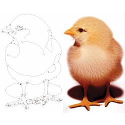
We vectorize the blur and color values with the same method as in Section 4.2. We sample colors in the direction normal to the polyline approximating each edge segment and apply the DouglasPeucker algorithm to obtain the color and blur control points. For an estimated blur σ, we pick the colors at a distance 3σ from the edge location, which covers 99% of the edge’s contrast, assuming a Gaussian blur kernel.8 While the 3σ distance ensures a good color extraction for the general case, it prevents the accurate extraction of structures thinner than 3 pixels (σ < 1). Figures 7 and 8 illustrate the result of the automatic conversion of a bitmap image into a diffusion-curve representation. The diffusion curves preserve the realistic look of the original photograph while offering the resolution independence of vector graphics representations.
Discussion: Several parameters determine the complexity and quality of our vectorized image representation. For the edge geometry, the Canny threshold determines how many of the image edges are to be considered for vectorization; a despeckling parameter sets the minimum length of a pixel chain to be considered for vectorization; and finally, two more parameters set the smoothness of the curve fitting and the fitting error. For the blur and color values, two parameters are considered: the size of the neighborhood for eliminating outliers, and the maximum error accepted when fitting the polyline. We refer the interested reader to our original paper21 for the exact values of these parameters and to Section 6 for a discussion on image compression.
5. Results
Diffusion curves, as vector-based primitives, benefit from the advantages of traditional vector graphics: zooming-in preserves sharp transitions (Figure 8 (c)) and keyframe animation is easily performed via linear interpolation of geometry and attributes (Figure 5(e)).
To validate our approach and to collect valuable practical feedback, we had various artists use our prototype. Most figures in this paper were generated in these sessions. All artists were well versed in digital content creation tools, but had no technical background. They were given a brief tutorial, amounting to approximately 10 minutes of instruction. The artists were able to create many varied and intricate examples from the first session. Artists also appreciated the similarity between our tool and the traditional line drawing workflow, allowing them to gradually create their artwork by adding lines and colors. In contrast, gradient meshes require careful planning and a good understanding of the final composition of the intended art piece. Manual image creation took anywhere from several minutes (Figure 6) to a few hours (Figures 5 and 9(a)). However, the artists agreed that manipulating curves and colors with control points takes time and a more direct manipulation through over-sketching and painting would greatly speed up the creation process.
We provide in Figure 10 a visual comparison between diffusion curves and gradient meshes. In terms of sparsity of encoding, both gradient meshes and diffusion curves are very efficient image representations. A direct comparison between both representations is difficult, as much depends on the chosen image content, the desired level of realism, the economy with which artists draw, or the performance of the automatic conversion algorithm. The diffusion curves representation appears more compact at first glance as it only stores information at image boundaries, while gradient meshes often need to subdivide smooth regions. However, each geometric curve can hold an arbitrary amount of color and blur control points (see Table 1) while gradient meshes only store colors at vertices. So, while the sparsity of encoding of both representations is comparable, the flexibility of diffusion curves allows any degree of control on a curve, without a topologically-imposed upper or lower bound on the number of control points.
In some situations, the limited spatial extent of gradient meshes can be useful, for example when moving a gradient mesh to a different part of an image, or when warping the entire mesh. Such manipulations are also possible in our representation, but not as straightforward. In order to move parts of an image, the relevant curves have to be selected and moved as a unit. More importantly, without support for layering and transparency (see Section 6) it is difficult to ascertain how the colors of outer edges should interact with their new surroundings. A mesh warp could be implemented as a space warp around a group of curves.
6. Discussion and Future Work
We have introduced diffusion curves as a new image representation, offering most of the benefits usually found in vector approaches, such as resolution independence, geometric editability, and compactness; while at the same time allowing for highly complex image content, previously only realizable with raster graphics.
It is noteworthy that several future challenges discussed in our original paper20 have since been addressed. As diffusion curves are a non-layered, planar map representation, Bezerra et al.2 modified how constraints are expressed and evaluated between diffusion curves, thereby improving their behavior at intersections between curves. A more involved, but also more powerful and smoother solution, consists in using bi-harmonic instead of harmonic interpolation. This requires a specific solver, such as the one proposed by Finch et al.10
However, despite these and other extensions, some practical limitations still exist. Diffusion curves rely on the global solution to a (bi-)harmonic equation, an expensive operation that is feasible for interactive use only on a powerful GPU system.11,20 While such a system may be reasonably assumed for creation and editing, it should not be required for a viewing application, especially considering the increasing ubiquity of document consumption on power-limited mobile devices.
One solution has recently been proposed by Boyé et al.3: they provide a dedicated solver for (bi-)harmonic equations from curve and point constraints, which relies on finite-element methods (FEM). Here, the domain is not divided into a regular pixel-grid, but into a content-guided triangulation of the image. Note that this approach is different from gradient meshes, since the triangulation is not manipulated directly but dynamically updated by the solver. Using a triangulation approach, the diffusion curves are first inserted as triangulation constraints and then the remaining domain is subdivided to achieve a user-specified quality measure (minimum area, minimum angle, maximum edge-length, etc.) Once the domain is sufficiently triangulated, the diffusable attributes are set as constraints on the diffusion curves’ vertices and interpolated on all other vertices using a suitable FEM solver. The result of these operations is a triangulated image with color values at each vertex, which may be exported into any popular vector format.
Note that the above approach may diffuse color and blur values, but it does not implement the post-blurring operation, itself a rather expensive process. As such, another useful extension to diffusion curves would be to implicitly apply the blurring as part of the diffusion process, instead of an explicit post-process.
While our conversion algorithm is simple, it does not guaranty that the resulting set of curves is optimal for compression purposes, that is, that it is the smallest set of curves that can achieve a given quality. Using diffusion curves for image compression would likely require a global optimization approach as well as a more efficient data structure to exploit redundancy in curve position and color. However, minimum file size is not the only criteria for a successful conversion algorithm, as editability should also be taken into account for computer graphics applications.
Acknowledgments
We would like to thank Laurence Boissieux and Philippe Chaubaroux for the time they spent testing our prototype and for the artwork they created with it. We would also like to thank the anonymous reviewers, and all the people from Adobe and INRIA for their constructive comments and feedbacks. Alexandrina Orzan was supported by a grant from the European Community under the Marie-Curie Action MEST-CT-2004-008270.
Figures
 Figure 1. Diffusion curves (left), and the corresponding color image (right). Note the complex shading on the folds and blur on the face.
 Figure 2. Raster graphics have a finite resolution, producing visual artifacts when magnified too much. Vector graphics can be magnified artifact-free.
 Figure 3. A Diffusion curve is composed of (a) a geometric curve described by a Bézier spline, (b) arbitrary colors on either side, linearly interpolated along the curve, (c) a blur amount linearly interpolated along the curve. The final image (d) is obtained by diffusion and reblurring. Note the complex color distribution and blur variation defined with a handful of controls.
 Figure 4. Rendering diffusion curves requires (1) the rasterization of the color and blur sources, along with the gradient field w = (wx, wy), (2) the diffusion of colors and blur, and (3) the reblurring of the color image.
 Figure 5. Example steps for manual creation: (a) sketching the curves, (b) adjusting geometry, (c) setting color and blur, (d) final result, and (e) keyframe animation. The image (d) was created in 4 hours by an artist at first contact with the tool.
 Figure 6. Tracing with diffusion curves (artist drawing time: 90 minutes): (a) original bitmap, (b) tracing with active contours, and (c) diffusion curves.
 Figure 7. Automatic vectorization of a bitmap image: (a) original bitmap, (b) automatic vectorization, (c) diffusion curves, and (d) RGB difference (amplified by 4). Note that the most visible error occurs along edges (d), most probably because, through vectorization, we change their location.
 Figure 8. Automatic vectorization: (a) original bitmap, (b) vectorization, and (c) magnification of (b).
 Figure 9. Additional results created manually (a) and automatically (b).
 Figure 10. Comparison with gradient mesh. The gradient mesh (b) is composed of 340 vertices, and as many color control points (© Brooke Nuñez Fetissoff http://lifeinvector.com/). The Diffusion curves image (c) is composed of 38 curves, with 365 geometric, 176 left-color, and 156 right-color control points. (a) denotes the original photograph.


Join the Discussion (0)
Become a Member or Sign In to Post a Comment